Exhaust Port Challenge

1. Aim, Introduction, Theory:

The prime objective is to perform and verify the numerical simulation of four cylinder diesel engine exhaust port using Ansys fluent 2020 R2 version. The conjugat heat transfer anlysis has been carried out in order to check the heat transfer characteristics of exhaust port subjected to convective heat transfer boundary condition at its outer surface. The hot gases after combustion flows through four different inlets with a velocity of 5m/s and exhuatsed out from the outlet port with higher velocity. The gases enters the inlet port with a temperature of 700K. Different turbulence models are studied to verify the results and to plot the various velocity and temperature contours. The convective heat transfer coefficient near the wall is also determined and plotted. The major changes in the value of velocity, wall convection, and temperature is observed in the bend of exhuast port.

The three fundamental modes of heat transfer are Conduction, Convection and Radiation. The heat always transfer from a region of high temperature to region of low temperature. There are certain situations where both solid and fluid domain comes in contact with each other under such condition the mode of heat transfer by conduction in solid and convection in fluid are coupled at the interface of both solid and fluid, such coupled mode of heat transfer problems are called as conjugate heat transfer (CHT).There are wide areas of CHT applications such as conjugate heat transfer phenomenon in heat exchanger, solar heaters, Nuclear fuel elements, automobile radiators, electronics cooling system, and battery thermal management system etc.

2.Solving & Modelling approach:

A exhaust port basically consists of four inlet port and one outlet port. The diameter of all the inlet port is constant and the inlet velocity and temperature of hot gases are 5m/s and 700K respectively. The exhaust port is maintained at zero gauge pressure, while the outer wall of the exhaust pipe is subjected to convective heat transfer coefficient of 20W/m^2 K with air as a fluid having free stream temperature of 300K.

Initialy a base line mesh is generated both in solid and fluid domain using tetrahedral mesh. Then the required boundary conditions are applied on the model. The varoius required results are plotted, again the mesh is refined by adding inflation layers and reducing the element size both in fluid and solid domain in order to capture the wall convective coefficient.

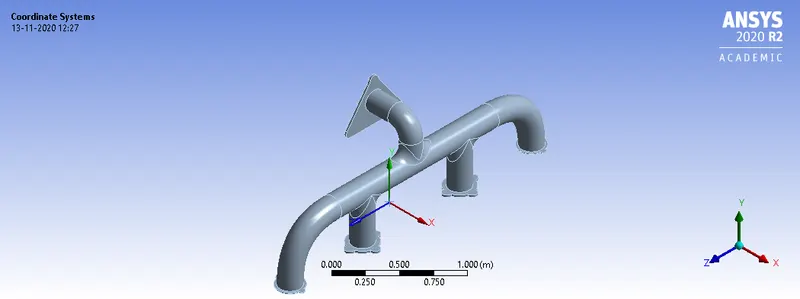
Figure 1. Exhaust Port Model.

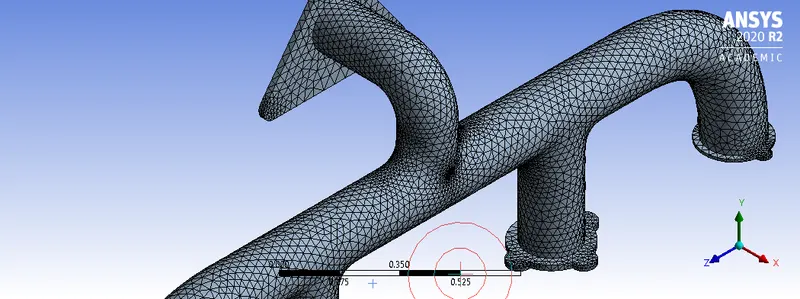
Figure 2. Base Line Mesh.

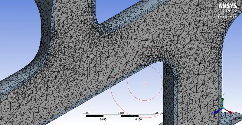
Figure 3. Sectional view of base line mesh.

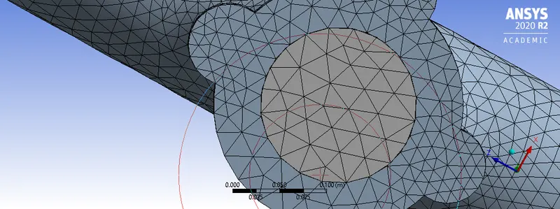
Figure 4. Non conformal mesh between solid and fluid domain.

A non conformal mesh is one in which the elements or faces of mesh in solid domain do not match with that of in fluid domain due to which an imperfect region of mesh is seen at the interface of solid and fluid bodies which is as shown in the above figure 4.

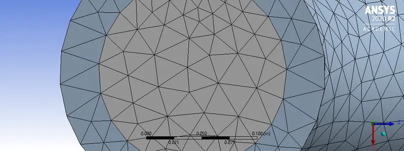
Figure5. Conformal Mesh.

To overcome the problem of non conformal mesh try to use share topology tool and in workbench click on share prep. This will helpful in converting the nonconformal regioninto conformal one.

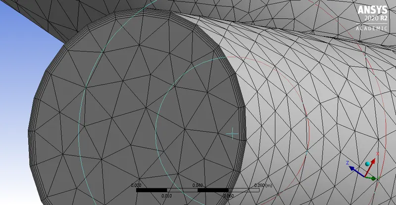
Figure 6. Inflation Layers.

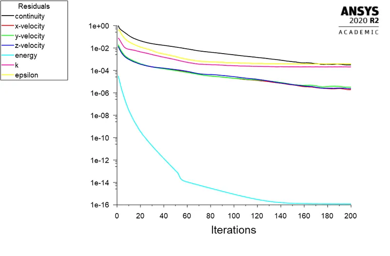
Fifure 6 (a). Residual plot for base line mesh (K-epsilon model).

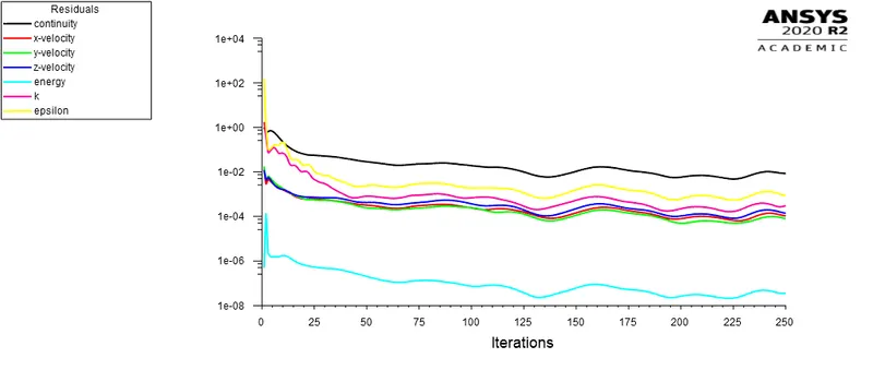
Figure 6(b): Residual Plot for refined mesh K-epsilon model.

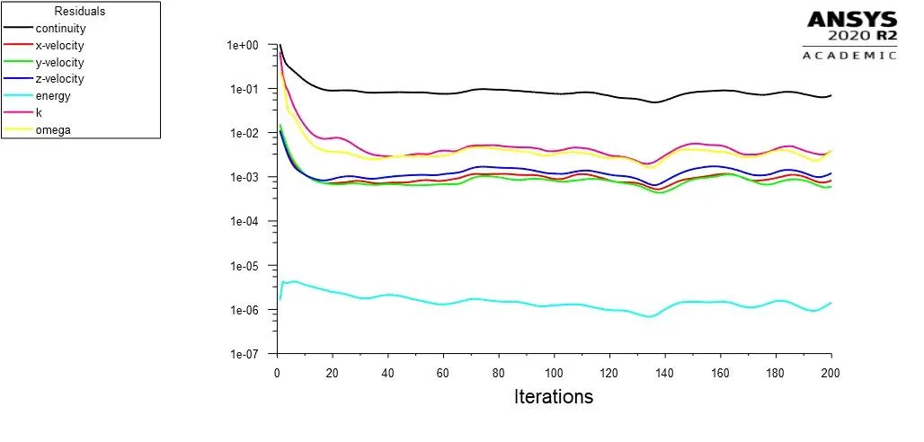
Figure 6 (c): Residual plot for refined mesh (K-Omega model)

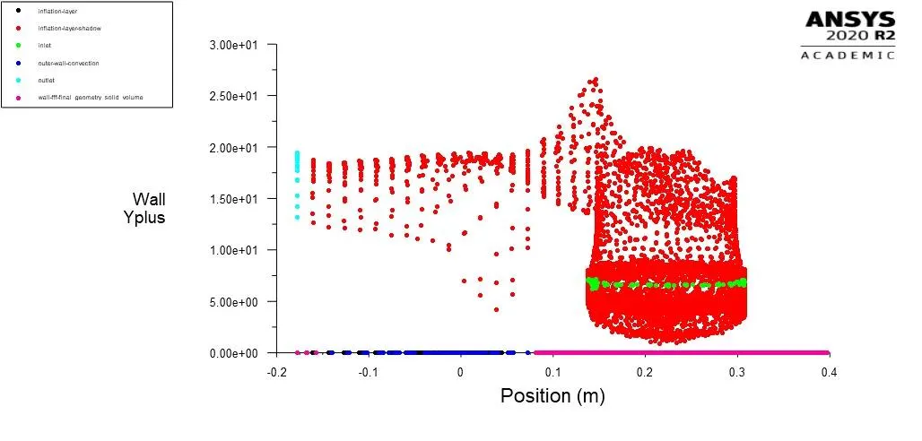
Figure 6(d): Y+ for refined mesh (K-epsilon Model).

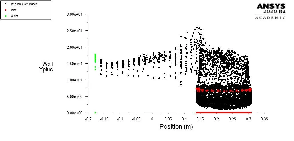
Figure 6(e): Y+ for refined mesh (K-omega model)

3. Pre-processing and solver setting:

In pre-processing step the physics of the given problem and approparite boundary conditions should be predefined before initilizing the solution. Once the physiques is set the solution is initilized and run for predefined iterations in order to obtain the converged solution.

Solver Settings:

Solving Method: Steady state, Pressure based solver

Viscous Model: Turbulence model, K-epsilon model, K-omega model (SST)

Energy equation:ON

Solving Scheme: Coupled Scheme

Material Used:

Fluid: Air

Solid: Aluminium

Boundary Conditions:

Inlet (Velocity, Temperature): 5m/s, 700K

Outlet (Pressure): Zero gauge pressure (Atmospheric pressure)

Outer wall: Convective heat transfer coefficient (20 W/m^2 K)

Free stream Temperature (Air) : 300K

4. Results:

Case1: Base Line Mesh (K-Epsilon Model):

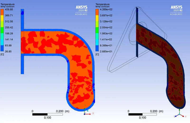
Figure 7. Temperature contours at outlet port.

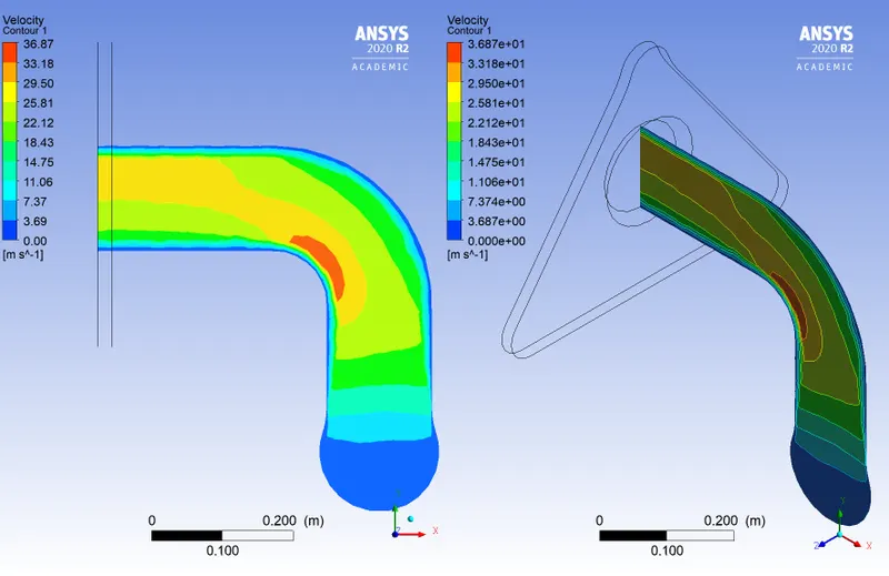
Figure 8. Velocity contours at outlet port.

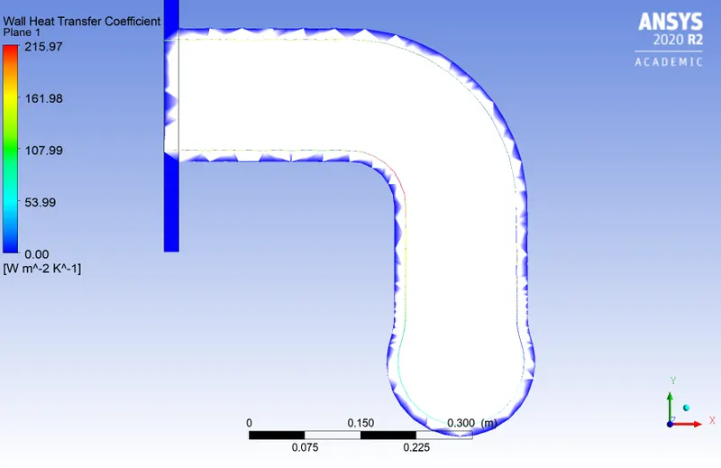
Figure 9. Wall Convective HTC.

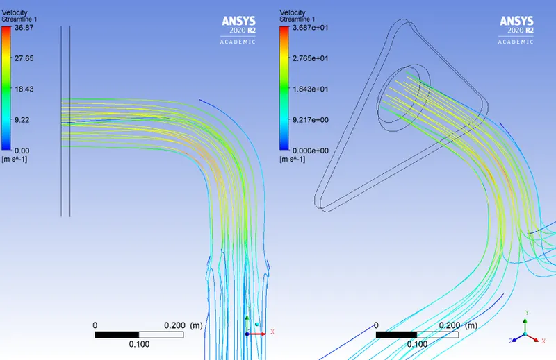
Figure 10. Velocity Streamlines.

Case 2: Refined Mesh (K-epsilon Model)

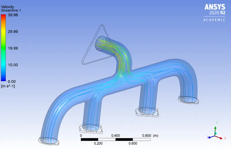
Figure 11. Velocity Stream Lines.

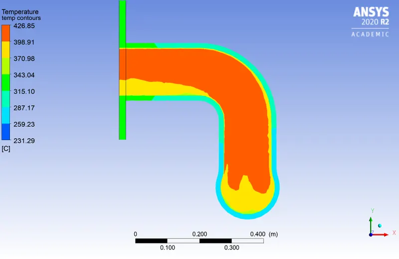
Figure 12. Temperature contours.

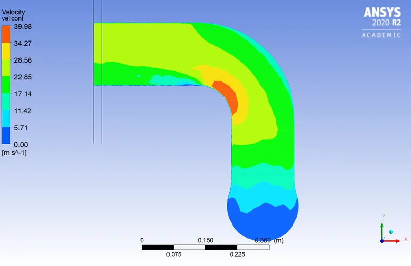
Figure 13. Velocity contours.

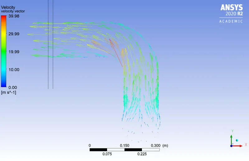
Figure 14. Velocity vectors.

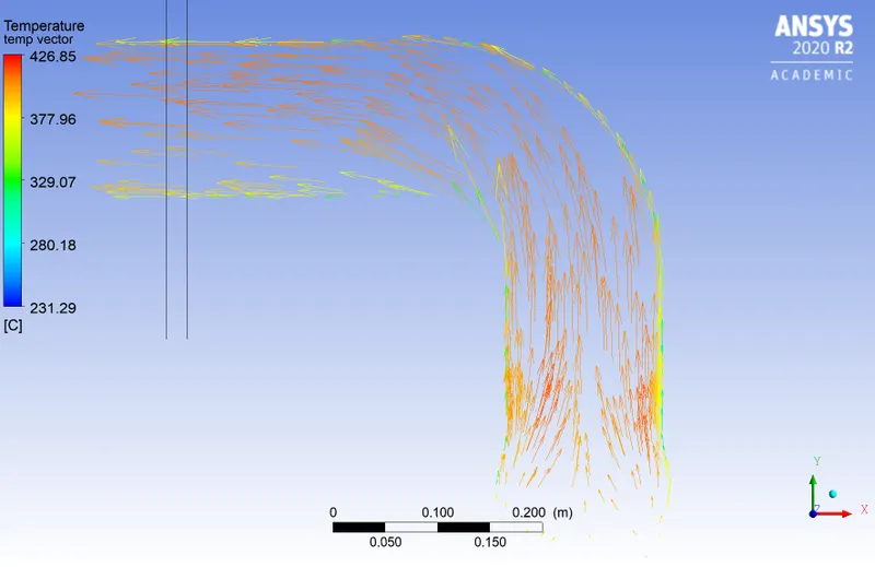
Figure 15. Temperature vectors.

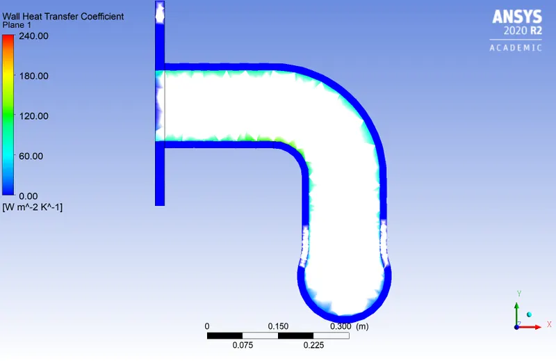
Figure 16. Heat transfer coefficient.

Case3: Refined Mesh (K-omega Model)

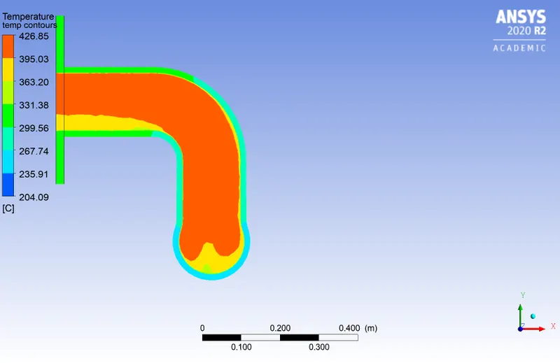
Figure 17. Temperature contours.

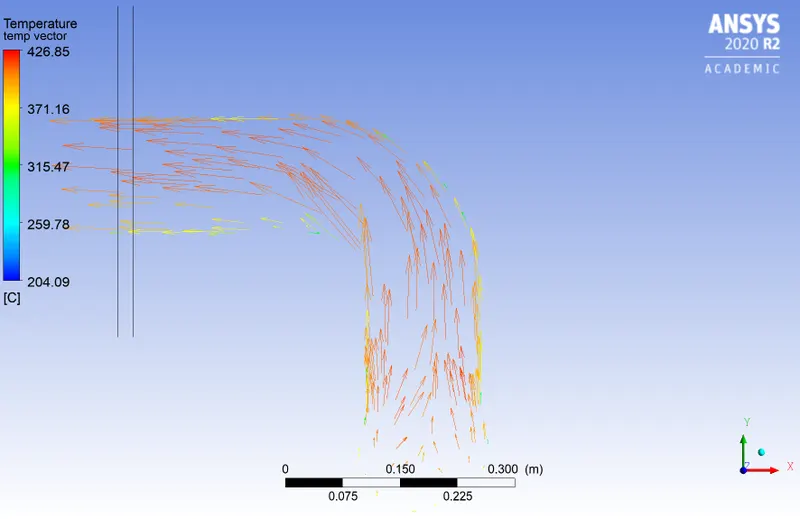
Figure 18. Temperature vector.

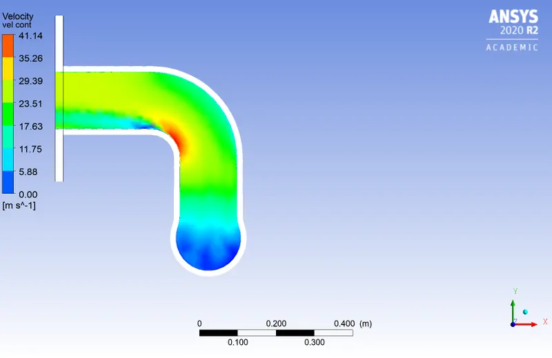
Figure 19. Velocity contours.

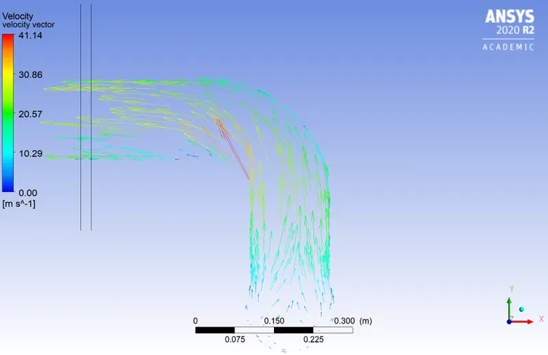
Figure 20. Velocity vectors.

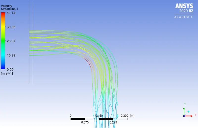
Figure 21. Velocity streamlines.

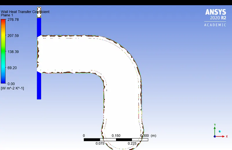
Figure 22. Heat transfer coefficient.

5. Conclusion:

From the above plotted results the following conclusions can be made

• The base line mesh doen not give accurate results.
• The K-epsilon and K-omega model proves to good and efficient in studying the turbulence behavoiur of fluid.
• For both the turbulence model the sharp rise in velocity of air is observed at the outlet port and reaches a value of upto 40 to 41 m/s.
• The maximum heat transfer coefficient is recorded in the region where the velocity is high.
• From temperature and velocity contour plots it is observed that the region where the velocity is less the corresponding temperature in that region is also less.
• The convective heat transfer coefficient is dependent on velocity of fluid.
• Maximum conjugate heat transfer is recorded in the region where the HTC is maximum.
• Small variation is observed in Y+ value for both K-epsilon and K-omega turbulence model.