1 D Linear Convection Problem - Numerical Solution to Wave Equation

The linear convection is the problem we involves the following equation,

`(∂u)/(∂t)+ c.(∂u)/(∂x)=0`

By converting this equation into analytical format, we use the taylor series expansion, where by applying the First order Forward diffencing with first order error to the time derivative term we use the equation. As as we need to compute the value of time at the future time step, we are using the forward time step.

`(∂u)/(∂t)= (u_i^(n+1)- u_i^n)/(Δt)`

Simillary the equation of space is converted to analytical form, by applying the First order Backward Differencing with first order error, we use the equation. And this equation is explicit approach. As the boundary conditions at the left side is know to us, we can apply the backward difference scheme to the space equation

`(∂u)/(∂x)= (- u_(i-1)^n+ u_i^n)/(Δx)`

By combining the two equations of analytical form, we get the generalised equations like

`u_i^(n+1)=u_i^n+ (-(c*Δt)/(Δx))*(- u_(i-1)^n+ u_i^n)`

By using this equation, we solve the problem by taking the constant of

L = 1m, Initial velocity is kept as a step function, between x=0.1 and x=0.3, the velocity is 2m/s and rest all the places the velocity is 1m/s. The value of C = 1, step time is kept as 0.01 sec. And by varing the value of number of grid (mesh size) of 20, 40, 80 and 160, the different observation are made.

And Based on the Von-Neumann approach to the Stability analysis, the courant number is derived. And the Courant number governs the stability or unstability of the convection equation using the explicit method. The Courant Number is represented by the formula, which is generally referred to as Courant–Friedrichs–Lewy(CFL). And most explicit one-dimensional advection schemes need to satisfy the condition that the Courant number, must be less than or equal to 1, for more stable in the von Neumann sense

`CFL = c*(dt/dx)`

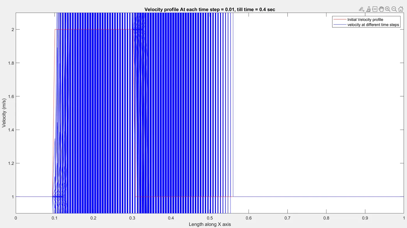
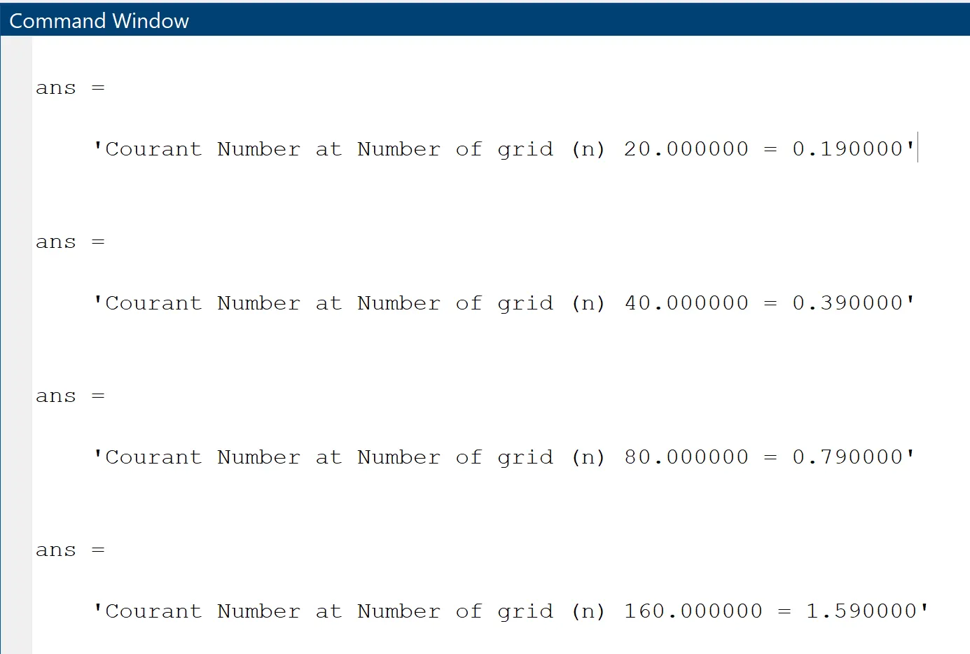
The value of Courant Number is calculated for every different value of number of grid size. As the finer the mesh size with constant time step, yields higher courant number and the solution is completely unstable as we can see from the results of n = 160.

This the matlab Code used for solving the problem.

clc;
close all;

L  = 1;     % Length
c  = 1;     % constant in the linear convection
dt = 1e-2;  % Time Step = 0.01

for n=[20 40 80 160]            %  n  =  Number of Grid points
    %% Calculations of Mesh
    x = linspace(0,L,n);
    dx=x(2)-x(1);   % or dx=L/(n-1)
    n_start=1;
    n_stop=1;
    
    %% Define the start and end position of the square wave
    for value=1:length(x)
        if((round(x(value)*n)/n==0.1)&&(rem(n_start, n_start)==0))
            n_start = value;
        end
        if((round(x(value)*n)/n==0.3)&&(rem(n_stop, n_stop)==0))
            n_stop  = value;
        end
    end

    %% Initialize Arrays and apply boundary conditions
    u = ones(1,n);
    u(n_start:n_stop)=2;

    nt = 40;                       % Number of Time steps
    uold = u;
    u_initial = u;

    %% Time Loop
    for k=1:nt
        % Convection Equation du/dt = -c*du/dx
        for i=2:n
            u(i) = uold(i) - (c*dt/dx)*(-uold(i-1)+uold(i));  
            % First Order Forward Differencing with first order error - Time derivative 
            % (u2(n+1))-u2(n))/(dt)
            % First order Backward Differencing with first order error - space Term 
            %(-u2(i-1)+u2(i))/(dx)
         end

        % Update old velocity
        uold = u;
        %Plotting the velocities
        figure(n);
        plot(x,u_initial,'color','r')
        hold on
        plot(x,u,'color','b');
        axis([0 1 0.9 2.1]);
        title('Velocity profile At each time step = 0.01, till time = 0.4 sec');
        xlabel('Length along X axis');
        ylabel('Velocity (m/s)');
        pause(0.003);
        legend('Initial Velocity profile','velocity at different time steps') 
    end
    
    Courant_Number=c.*dt./dx;
    sprintf('Courant Number at Number of grid (n) %f = %f',n,Courant_Number)

end

From the Matlab Code , we will get 4 graphs which correspond to each value of n = [20,40,80,160]

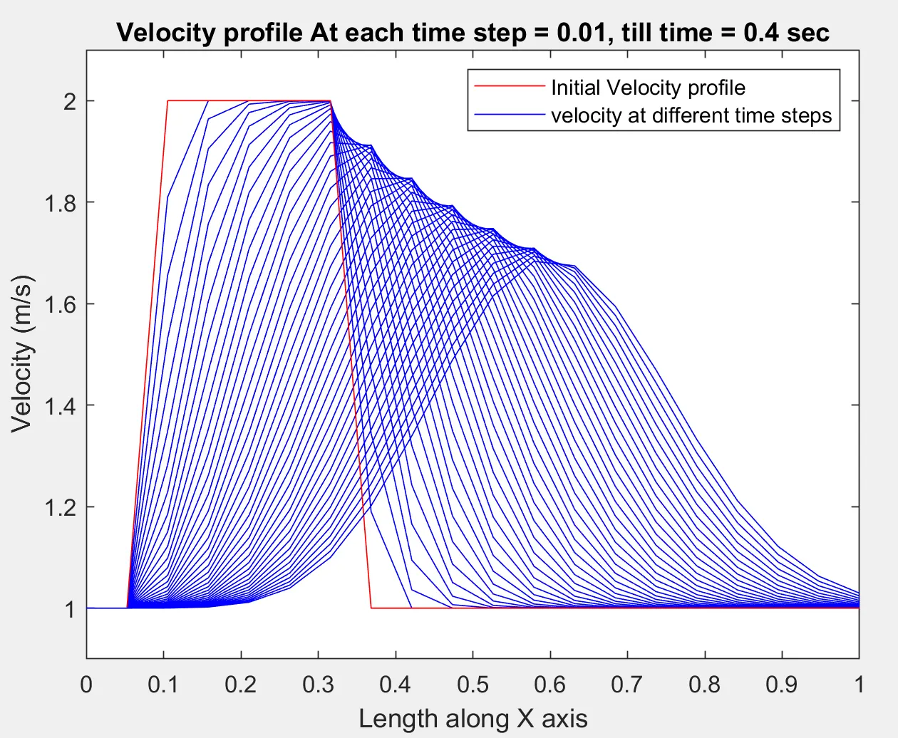
for number of nodes = 20, we get the profile like this. The profile drops down, and it is due to the phenemon of artificial diffusion also called as false diffusion.

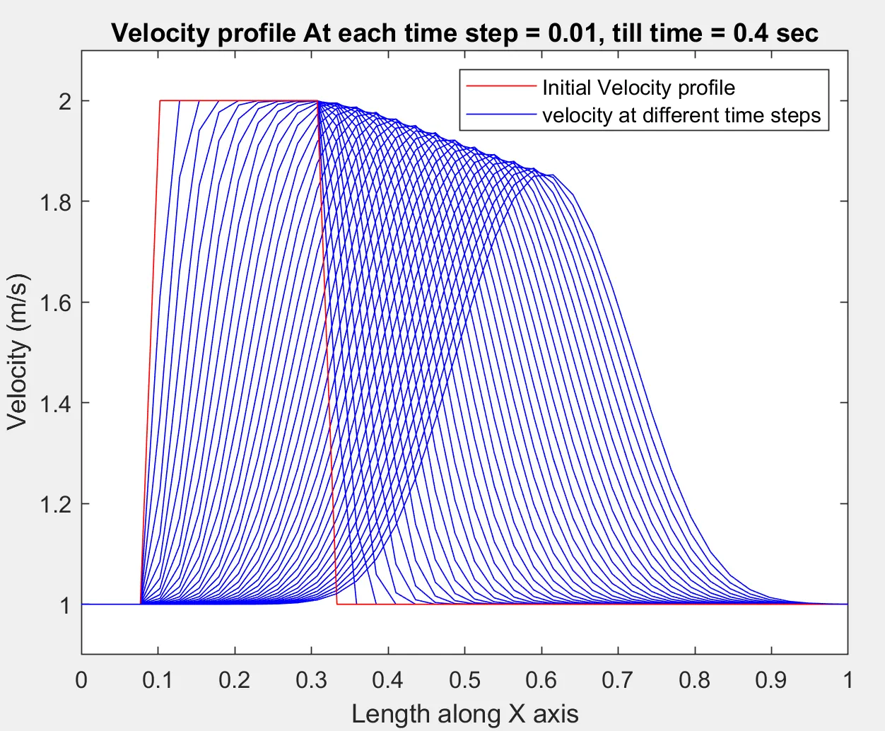
for number of nodes = 40, we get the profile like this.

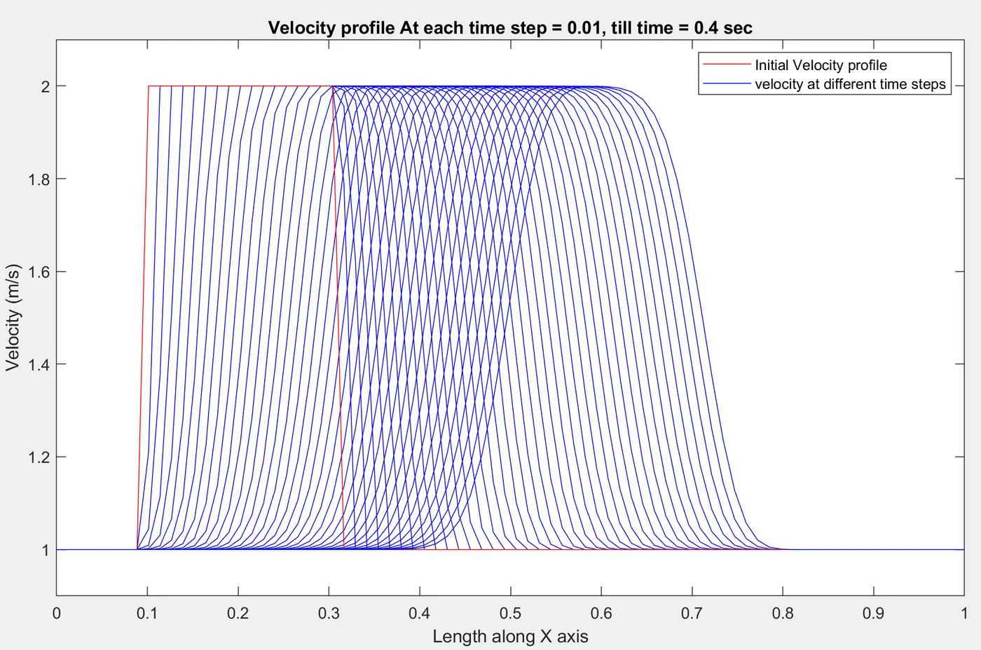
for number of nodes = 80, we get the profile like this. Only for this profile we can conclude that the initial value is propagated to the final position without any artificial diffusion.

for number of nodes = 160, we get the profile like this. Here too much wiggles are observed, and this is due to the Gibbs Phenemenon.

NOTE:

1. The solution for n=160 , is completly unstable as the courant number is greater than 1.

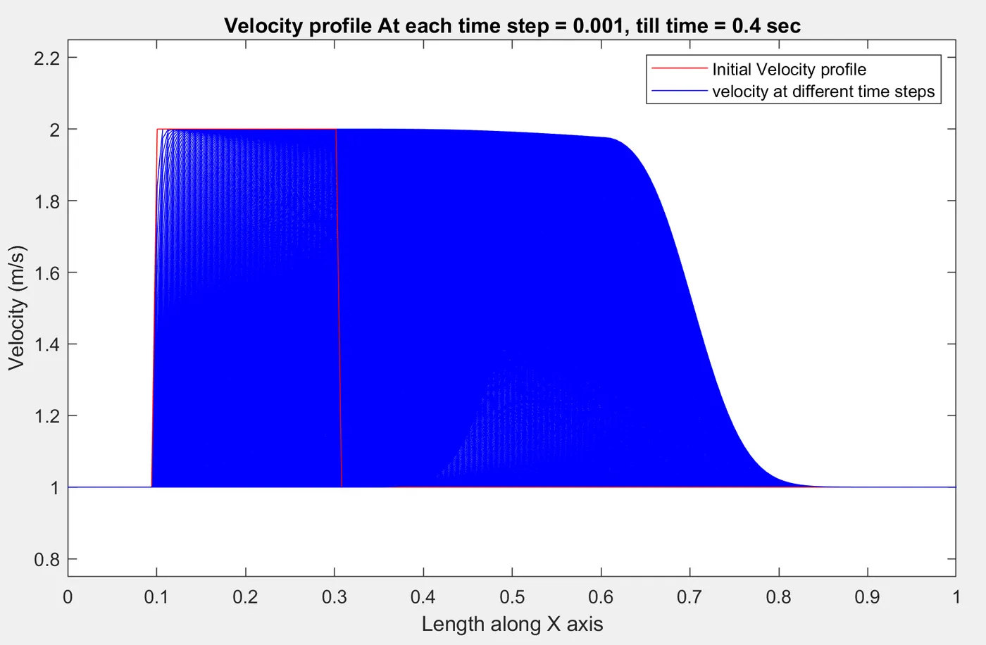
2. The profile of the curve velocity at various time step is lost at the end of time = 0.4 sec, due to the presence of artificial diffusion. This is also called as false diffusion. This is generally a type of error observed when the analytical method is used to approximate the convection term in convection–diffusion equations. This type of error can be found minimised for the value of n = 80.

3. When the value of dt is changed by fixing the value of the time as t = 0.4 sec, for n = 160, dt = 0.001, we get the following profile, where the pofile is smothly travelling along the x axis. The courant number observed here is 0.1590. Thus the courant number is very critical in providing the stable solution.

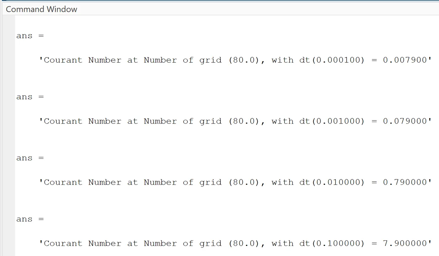
4. By keeping the value of number of grid (n) =80, L =1m, C = 1, between the values of x ranging from 0.1 to 0.3, the velocity is 2m/s and remaining position of x the velocity is 1m/s. And the value of dt is being kept in a for loop with steps of 1e-4, 1e-3, 1e-2, and 1e-1. Based on the value of dt, the number of times the time equation is being solved in the for loop is changed by using the formula given below. As we need to find at time = 0.4sec, the total simulation is being run. The matlab code is shown below.

`nt = 0.4/dt`

clc
close all

L  = 1;     % Length
c  = 1;     % constant in the linear convection
n = 80;     %  n  =  Number of Grid points

for dt=[1e-4 1e-3 1e-2 1e-1]            % dt = time step
    %% Calculations of Mesh
    x = linspace(0,L,n);
    dx=x(2)-x(1);   % or dx=L/(n-1)
    n_start=1;
    n_stop=1;
    
    %% Define the start and end position of the square wave
    for value=1:length(x)
        if((round(x(value)*n)/n==0.1)&&(rem(n_start, n_start)==0))
            n_start = value;
        end
        if((round(x(value)*n)/n==0.3)&&(rem(n_stop, n_stop)==0))
            n_stop  = value;
        end
    end

    %% Initialize Arrays and apply boundary conditions
    u = ones(1,n);
    u(n_start:n_stop)=2;

    nt = 0.4/dt;                       % Number of Time steps
    uold = u;
    u_initial = u;

    %% Time Loop
    for k=1:nt
        % Convection Equation du/dt = -c*du/dx
        for i=2:n
            u(i) = uold(i) - (c*dt/dx)*(-uold(i-1)+uold(i));  
            % First Order Forward Differencing with first order error - Time derivative 
            % (u2(n+1))-u2(n))/(dt)
            % First order Backward Differencing with first order error - space Term 
            %(-u2(i-1)+u2(i))/(dx)
         end

        % Update old velocity
        uold = u;
        
    end
%       Plotting the velocities
    figure(1);
    plot(x,u);
    axis([0 1 0.9 2.1]);
    xlabel('Length along X axis');
    ylabel('Velocity (m/s)');
    title('Velocity profile at t = 0.4 sec at different with dt')
    hold on;
    Courant_Number=c.*dt./dx;
    sprintf('Courant Number at Number of grid (%0.01f), with dt(%1f) = %f',n,dt,Courant_Number)
end
figure(1);
plot(x,u_initial,'color','k');
legend('dt = 1e-4','dt = 1e-3','dt = 1e-2','dt = 1e-1','Initial Velocity')

And for each value of dt, the courant number is varied. At dt <=0.01, the solution is better and the initial velocity profile is moving along the direction of x, without much significant loss of artificial diffusion. But at dt = 0.1, the courant number is 7.9, which gives completely unstable results and at the end it gives rise to wiggles. This is due to the phenemenon of gibbs phenemon.

The velocity profile at the end of the simulaiton till the time of 0.4 sec, for various values of time step is shown below.

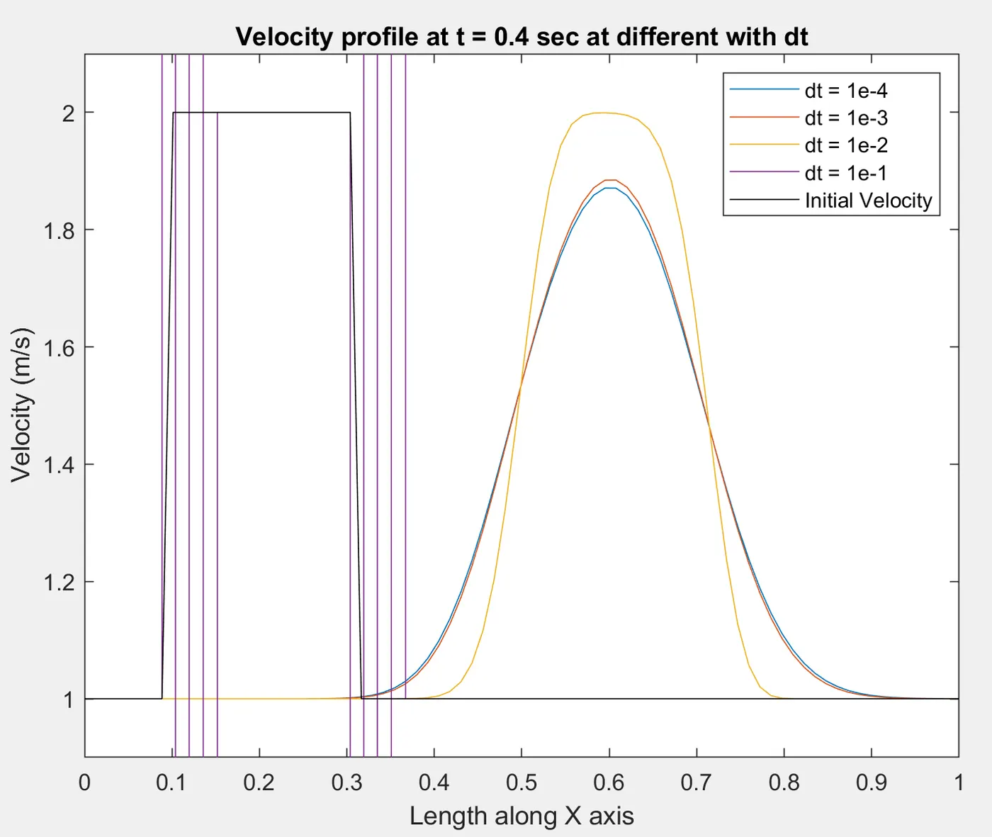
From the profile of the graph we can conclude that for very small values of dt, the velocity profile is lost along the direction of x. This loss is due to the artificial diffusion. But if the value of dt=1e-2, the velocity profile is closely matching with the initial velocity with slight losses in the profile curvature. But at the value fo dt=1e-1, the velocity profile is completly mismatching with the initial velocity profile, this is due to the phenomenon called as gibbs phenomenon. Even at this value of dt, if we try to decrease the value of dx, the CFL number reduces, and it will give better results, but this results will not be able to capture the physics accurately. So it is better not to use higher values of dt.