Taylor table method - Second order Derivative with 4th order Accuracy Using - Central Difference, Skewed right-sided difference and Skewed left-sided difference - Using Matlab
The approximation of the numerical derivative with the analytical derivative can be done with the help of Taylor Table method. Where the expansion of the f(i-1), f(i-2), f(i+1), f(i+2).. etc can be done with the help of taylor series method and then by equating the quotients, we can get the value of the unknowns.
The function used for performing this function is
`exp(x)*cos(x)`
The analytical derivative of this function is given as
syms x
g=exp(x).*cos(x);
diff(g,2)
Second order Derivative of the function is
`-2*exp(x)*sin(x)`
So inorder to perform the numerical derivative of the function using matlab we follow different approaches like central differencing, forward differencing and backward differencing.
1. Central Differencing - with 4th order accuracy
The number of terms of the central differencinng of the second order derivative with the 4th order accuracy can be determined by using the formula
`p + q - 1`
where p = order of the derivative,
q = order of accuracy
here, p = 2, q = 4 , therfore the number of terms = 2 + 4 - 1 = 5 . It can be writted of the form
`(d^2 y)/(dx^2) = (a*f(i-2)+b*f(i-1)+c*f(i)+d*f(i+1)+e*f(i+2))/(Δx)^2`
By expanding each and every terms using the taylor series form we can obtain this table, using this table we can find the co-efficients like a,b,c,d and e. By solving the system of equations from Taylor table method, we get 5 equations with 5 unknown,
| Numerical Stensil | f(i) | `Δx.f'(x)` | `(Δx)^2*f^(II)(x)` | `(Δx)^3*f^(III)(x)` | `(Δx)^4*f^(IV)(x)` |
| `a*f(i-2)` | a | -2a | 4a/2 | -8a/6 | 16a/24 |
| `b*f(i-1)` | b | -b | b/2 | -b/6 | b/24 |
| `c*f(i)` | c | 0 | 0 | 0 | 0 |
| `d*f(i+1)` | d | d | d/2 | d/6 | d/24 |
| `e*f(i+2)` | e | 2e | 4e/2 | 8e/6 | 16e/24 |
| `Σ` | 0 | 0 | 1 | 0 | 0 |

A = [1       1  1  1     1;
    -2      -1  0  1     2;
     2     0.5  0 0.5    2;
    -8/6  -1/6  0 1/6   8/6;
   16/24  1/24  0 1/24 16/24];
B = [0;0;1;0;0];
C=AB

The value of C obtained is
C =

   -0.0833
    1.3333
   -2.5000
    1.3333
   -0.0833
2. Skewed right-sided difference - with 4th order accuracy
The number of terms of the skewed Right sided differencinng of the second order derivative with the 4th order accuracy can be determined by using the formula
`p + q`
where p = order of the derivative,
q = order of accuracy
here, p = 2, q = 4 , therefore the number of terms = 2 + 4 = 6 . It can be written of the form
`(d^2 y)/(dx^2) = (a*f(i)+b*f(i+1)+c*f(i+2)+d*f(i+3)+e*f(i+4)+f*f(i+5))/(Δx)^2`
So, this equation gives us 6 equations, with 6 unknows. The equations can be written from the table, and the equation can be solved using matrix multiplication.
`A X = B`
Using the matrix multiplication we can find the value of X, and the elements in the matrix X gives the values of a,b,c,d, e and f.
| Numerical Stensil | f(i) | `Δx.f'(i)` | `(Δx)^2*f^(II)(i)` | `(Δx)^3*f^(III)(i)` | `(Δx)^4*f^(IV)(i)` | `(Δx)^5*f^(V)(i)` |
| `a*f(i)` | a | 0 | 0 | 0 | 0 | 0 |
| `b*f(i+1)` | b | b | b/2 | b/6 | b/24 | b/120 |
| `c*f(i+2)` | c | 2c | 4c/2 | 8c/6 | 16c/24 | 32c/120 |
| `d*f(i+3)` | d | 3d | 9d/2 | 27d/6 | 81d/24 | 243d/120 |
| `e*f(i+4)` | e | 4e | 16e/2 | 64e/6 | 256e/24 | 1024e/120 |
| `f*f(i+5)` | f | 5f | 25f/2 | 125f/6 | 625f/24 | 3125f/120 |
| `Σ` | 0 | 0 | 1 | 0 | 0 | 0 |

Af=[1   1   1       1    1    1;
    0   1   2       3    4    5;
    0  1/2  4/2    9/2  16/2  25/2;
    0  1/6  8/6   27/6  64/6  125/6;
    0 1/24 16/24  81/24 256/24 625/24;
    0 1/120 32/120 243/120 1024/120 3125/120];
Bf =[0;0;1;0;0;0];
Cf=AfBf

The value of Cf is

Cf =

    3.7500
  -12.8333
   17.8333
  -13.0000
    5.0833
   -0.8333
3. Skewed left-sided difference
The number of terms of the skewed Right sided differencinng of the second order derivative with the 4th order accuracy can be determined by using the formula
`p + q`
where p = order of the derivative,
q = order of accuracy
here, p = 2, q = 4 , therefore the number of terms = 2 + 4 = 6 . It can be written of the form
`(d^2 y)/(dx^2) = (a*f(i-5)+b*f(i-4)+c*f(i-3)+d*f(i-2)+e*f(i-1)+f*f(i))/(Δx^2)`
So, this equation gives us 6 equations, with 6 unknows (a,b,c,d,e and f). The equations can be written from the table, and the equation can be solved using matrix multiplication
`A X = B`
Using the matrix multiplication we can find the value of X, and the elements in the matrix X gives the values of a,b,c,d, e and f.
| Numerical Stensil | `(Δx)^5*f^(V)(i)` | `(Δx)^4*f^(IV)(i)` | `(Δx)^3*f^(III)(i)` | `(Δx)^2*f^(II)(i)` | `Δx.f'(i)` | `f(i)` |
| `a*f(i-5)` | -3125a/120 | 625a/24 | -125a/6 | 25a/2 | -5a | a |
| `b*f(i-4)` | -1024b/120 | 256b/24 | -64b/6 | 16b/2 | -4b | b |
| `c*f(i-3)` | -243c/120 | 81c/24 | -27c/6 | 9c/2 | -3c | c |
| `d*f(i-2)` | -32c/120 | 16c/24 | -8c/6 | 4c/2 | -2c | d |
| `e*f(i-1)` | -d/120 | d/24 | -d/6 | d/2 | -d | e |
| `f*f(i)` | 0 | 0 | 0 | 0 | 0 | f |
| `Σ` | 0 | 0 | 0 | 1 | 0 | 0 |

For performing the derivative operation in matlab we have taken x = pi/3 and dx is varing from pi/4 to pi/4000
Ab = [ 1     1   1   1      1    1;
      -5    -4  -3   -2     -1    0;
      25/2  16/2     9/2     4/2    1/2   0;
     -125/6   -64/6    -27/6    -8/6   -1/6   0;
      625/24     256/24   81/24    16/24  1/24  0;
     -3125/120 -1024/120 -243/120 -32/120 -1/120 0];
Bb = [0;0;1;0;0;0];
Cb = AbBb

The value of Cb is
Cb =

   -0.8333
    5.0833
  -13.0000
   17.8333
  -12.8333
    3.7500
For performing the above operation the following lines of Code was used in matlab
clc
close all

%% Central Difference - Second order Derivative with 4th order accuracy

A = [1       1  1  1     1;
    -2      -1  0  1     2;
     2     0.5  0 0.5    2;
    -8/6  -1/6  0 1/6   8/6;
   16/24  1/24  0 1/24 16/24];
B = [0;0;1;0;0];
C=AB

%dx=pi/40;
dx=linspace(pi/4,pi/4000,80);
x=pi/3;
analytical_derivative=-2.*exp(x).*sin(x);
Central_differencing = (C(1).*(exp(x-2.*dx).*cos(x-2.*dx))+C(2).*(exp(x-dx).*cos(x-dx))+C(3).*(exp(x).*cos(x))+C(4).*(exp(x+dx).*cos(x+dx))+C(5).*(exp(x+2.*dx).*cos(x+2.*dx)))./(dx.^2);
Central_differencing_Error=abs(Central_differencing-analytical_derivative);
%% Skewed Right-Sided Difference (Forward Differencing)

Af=[1   1   1       1    1    1;
    0   1   2       3    4    5;
    0  1/2  4/2    9/2  16/2  25/2;
    0  1/6  8/6   27/6  64/6  125/6;
    0 1/24 16/24  81/24 256/24 625/24;
    0 1/120 32/120 243/120 1024/120 3125/120];
Bf =[0;0;1;0;0;0];
Cf=AfBf

Forward_Differencing = (Cf(1).*(exp(x).*cos(x))+Cf(2).*(exp(x+dx).*cos(x+dx))+Cf(3).*(exp(x+2.*dx).*cos(x+2.*dx))+Cf(4).*(exp(x+3.*dx).*cos(x+3.*dx))+Cf(5).*(exp(x+4.*dx).*cos(x+4.*dx))+Cf(6).*(exp(x+5.*dx).*cos(x+5.*dx)))./(dx.^2);
Forward_differencing_Error=abs(Forward_Differencing-analytical_derivative);

%% Skewed Left - Sided Difference (Backward Differencing)

Ab = [ 1     1   1   1      1    1;
      -5    -4  -3   -2     -1    0;
      25/2  16/2     9/2     4/2    1/2   0;
     -125/6   -64/6    -27/6    -8/6   -1/6   0;
      625/24     256/24   81/24    16/24  1/24  0;
     -3125/120 -1024/120 -243/120 -32/120 -1/120 0];
Bb = [0;0;1;0;0;0];
Cb = AbBb
Backward_Differencing = (Cb(1).*(exp(x-5.*dx).*cos(x-5.*dx))+Cb(2).*(exp(x-4.*dx).*cos(x-4.*dx))+Cb(3).*(exp(x-3.*dx).*cos(x-3.*dx))+Cb(4).*(exp(x-2.*dx).*cos(x-2.*dx))+Cb(5).*(exp(x-dx).*cos(x-dx))+Cb(6).*(exp(x).*cos(x)))./(dx.^2);
Backward_differencing_Error=abs(Backward_Differencing-analytical_derivative);

%% Plotting the errors
figure(1)
plot(dx,Central_differencing_Error,'Color','r');
hold on
plot(dx,Forward_differencing_Error,'Color','g');
hold on
plot(dx,Backward_differencing_Error,'Color','b');
xlabel('dx');
ylabel('Error');
legend('Central Difference Error','Skewed Right Error','Skewed Left Error')
title('Error vs dx')


figure(2)
loglog(dx,Central_differencing_Error,'Color','r');
hold on
loglog(dx,Forward_differencing_Error,'Color','g');
hold on
loglog(dx,Backward_differencing_Error,'Color','b');
xlabel('Log of dx');
ylabel('Log of Error');
legend('Central Difference Error','Skewed Right Error','Skewed Left Error')
title('Log (Error) vs Log(dx)')
For analying the results the plots of the error vs dx was plotted down
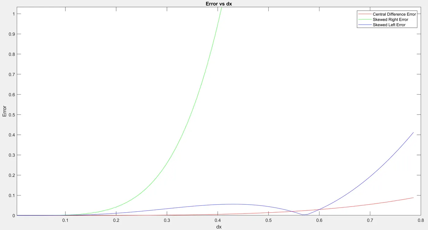
We can infer from the graph that the error for the skewed left showed very high error at the very small values of dx, i.e at finer mesh. but the errof for the central differencing is of the order of very very small compared with the forward and backward differencing method.
For analysing the results much more clearly, the log-log graph for the Error vs dx was plotted
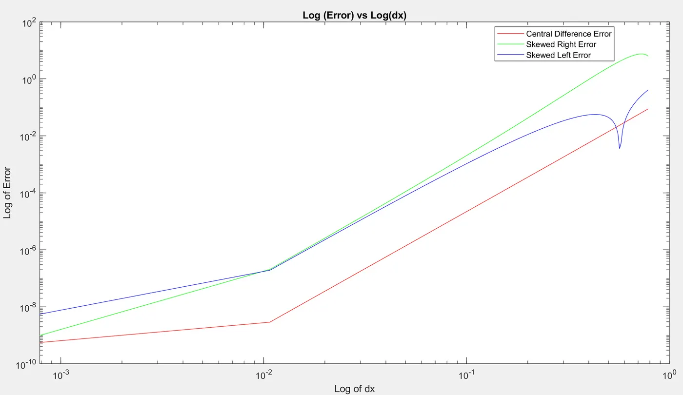
From this we can conclude that the central differencing will give the least error at most of the situations.
But skewed scheme is much more useful at many situations like at the corner nodes. Where all the information of i+1 and i+2 wont be available, so the CD cannot be used at such situations. Whereas the Skewed scheme can be used at all situations. For a rectangle block, at the left side the information of i-1, i-2 wont be available, so we can proceed with forward differencing(skewed right differencing). Whereas at the right side the information of i+1, i+2 wont be available, so we can proceed with the backward differencing (skewed left differencing).