Week 3 - Solving second order ODEs

Aim: To write program in Python to solve the System of 2nd Order Differential Equation(ODE) and to visualize the position of the simple pendulum at various instances of time. The ODE represent the equation of motion of a simple pendulum with damping.

Theory:

The ODE are generally used to solve the transient behaviour of a system.

Solution

The Algebric equation for the simple pendulum is shown below. And the numerical method to solve this equation can be done by using the Ordinary Differential equation approach. So we break the 2nd order ODE into 2 system of 1st order ODE equation as shown below. And by solving the two equations sperately we can determine the position and the velocity of the simple pendulum at various instances of time.

In the above equation the notations are

b= damping Coefficient

m=mass of the ball (kg)

g=gravity (m/s^2)

l= length (m)

By splitting the above equations we get the below 2 different equations.

`(∂θ_1)/(∂t)= θ_2` - (1)

`(∂θ_2)/(∂t)= -b/m θ_2-g/L sin⁡(θ_1)` - (2)

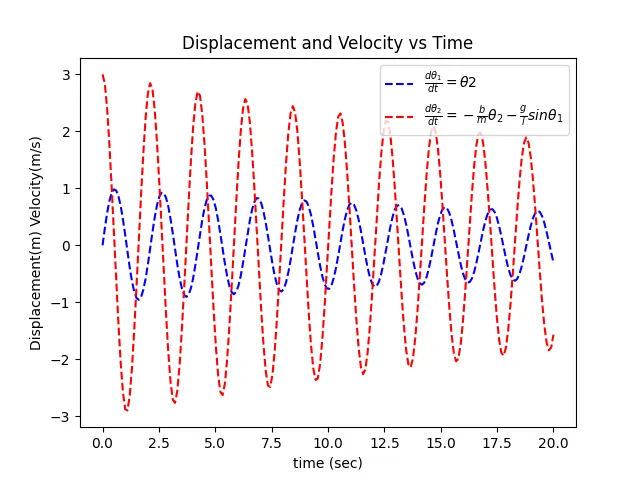
Equation 1 gives the value of displacement at various instances of time and Equation 2 gives the values of velocity.

The initial parameters are

l=1m, m=1kg, b=0.05, g=9.81 (m/s2)

and we simulate the motion between 0 to 20 sec, for angular displacement of 0, angular velocity of 3 rad/s2 at time t =0;

Python Code

import math
import matplotlib.pyplot as plt 
import numpy as np 
from scipy.integrate import odeint

# Function that return dz/dt
def model(theta,t,b,g,l,m):
	theta1=theta[0];
	theta2=theta[1];
	dt1=theta2;
	dt2=(-b*theta2/m)-(g*math.sin(theta1)/l)
	dt=[dt1,dt2]
	return dt

#Inputs
b=0.05;  # Damping Co-efficient
l=1; 	 # Gravity m/s2
g=9.81;	 # length of the pendulum in m
m=1;     # mass of the ball in kg

theta_0=[0,3]  # Initial conditions

# Time Points
t=np.linspace(0,20,200) #split from 0 to 20 into 200 points

#Solve ODE
theta=odeint(model,theta_0,t,args=(b,g,l,m)) #command in scipy module

#Plot
plt.plot(t,theta[:,0],'b--',label=r'$\frac{d\theta_1}{dt}=\theta2 $')
plt.plot(t,theta[:,1],'r--',label=r'$\frac{d\theta_2}{dt}=-\frac{b}{m}\theta_2 - \frac{g}{l}sin\theta_1 $')
plt.legend(loc='best')
plt.title('Displacement and Velocity vs Time')
plt.xlabel('time (sec)')
plt.ylabel('Displacement(m) Velocity(m/s)')
plt.show()

#Animation
ct=1;
x1=0;
y1=0;

for ang in theta[:,0]:
	x2=l*math.sin(ang)
	y2=-l*math.cos(ang)
	file='test%05d.png'%ct
	plt.figure()
	plt.plot([-1.5,1.5],[0,0],linewidth=8)
	plt.plot([x1,x2],[y1,y2],linewidth=3)
	plt.plot(x2,y2,'o',markersize=15)
	plt.xlim([-1.5,1.5])
	plt.ylim([-1.5,1.5])
	plt.savefig(file)
	ct=ct+1

Explaination of Code

1. The Scipy module is used to solved the ode equations (the odeint is used from scipy library)

2. The function named model is created to return the values of displacement and velocities [dt1 , dt2]. here dt1 represent the displacement and dt2 represent the angular velocities

3. The constants like damping coefficients, length, mass, gravity constant are instialized

4. The initlal condition angular displacement=0 to 3 rad/sec are initialized with theta_0

5. The linspace of numpy library splilts the number between 0 to 20 into 200 points

6. Then the displacement and velocities are ploted against time

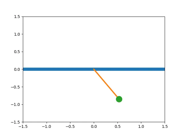
7. For animation a counter is created to save the file name as per the counter increases. And the figure is ploted for position at various instances of the angle. And each and every figure at various angles are being saved. And this saved images are being conveted into animation

Results and Discussion

1. Displacement and Velocity vs Time

The below graph plots the variation of displacement and velocity as a function of time. But due to the effect of damping co-efficient the variation between angular velocity and displacement changes over time occurs.

2. Animation for the Position of the Pendulum at various instances of Time

The below image shows the sample of the initial displacement of the simple pendulum at the initial point of time. As the time progress the simple pendulum tries to bring back to equibrilibum, so the displacement decreases over time. If we prolong the simulation upto 100 seconds, we would be able to find the stable position, so the simple pendulum reaches stability and rests.

The animation video is uploaded in the Google Drive as mentioned in the link below

https://drive.google.com/file/d/1aqIrnQ41DFiAdz-l3dwQztV7dtRmJaVv/view?usp=sharing