Week 2 Air standard Cycle

Aim:

To understand the principles of Otto cycle and to plot the pressure vs Volume curve using Python libraries. And to Determine the Thermal Efficiency of the Ideal cycle .

Theory:

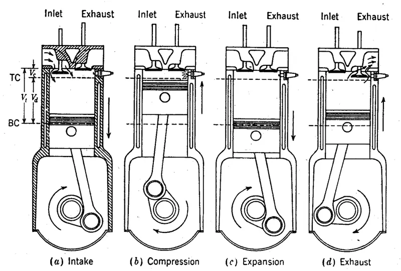
The Otto Cycle involves the 4 process

Step 1 :Compression

1 - 2 : Process 1 to 2 is an Adiabatic Compression (adiabatic and reversable hence isentropic compression)

Step 2: Combustion

2 - 3: Process 2 to 3 is constant Volume heat addition (Combustion occurs)

Step 3 : Expansion

3 - 4 : Process 3 to 4 is adiabatic expansion (adibatic and reversable)

Step 4 : Exhaust

4 - 1 : Process 4 to 1 is constant volume heat rejection

The Ideal Pressure vs Volume curve for Otto cycle is shown below

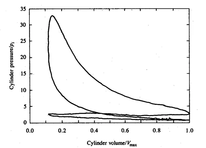
Equations

The Relation between the volume of the combustion chamber as a function of the crank angle is given below

- (1)

in the above equation, V = volume of combustion chamber

Vc = Clearance volume ,

rc = compression ratio,

theta = crank angle ,

a = crank radius = stroke length/2 (L=2a), B = Bore dia

R is the ratio of connecting rod length and crank radius

The Cylinder Volume at any crank position is given by

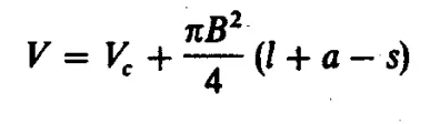- (2)

where s is the distance between crank axis and the piston pin axis

- (3)

By rearranging the 2nd and 3 rd equation we will be able to obtain the 1st equation.

The Equation for Thermal Efficiency of Otto cycle is

`η = 1/(r_c^(gamma-1) )`

Python Program:

The inputs that are used for plotting the graph are based on standard temperature and Pressure

Bore Dia (B) = 0.1m

Stroke Length (L)= 0.1m

Connecting Rod Length(l) = 0.15m

Compression Ratio (rc) = 8

Pressure at state 1 = 101325 Pa

Temperature at state 1 = 500 K

gamma (Ratio of specific heat at constant pressure and specific heat at constant Temperature) = 1.4

Temperature at state 3 (MAX. Temperature) = 2300K

'''
 	Otto Cycle Simulator
'''

import math
import matplotlib.pyplot as plt

def engine_kinematics(bore,stroke,con_rod,cr,start_angle,end_angle):

	#Engine Parameters
	a=stroke/2
	R=con_rod/a
	#Volume Computation
	v_s=(math.pi/4)*pow(bore,2)*stroke # Stroke Volume
	v_c=v_s/(cr-1)						# Clearance Volume
	
	sc=math.radians(start_angle) # Start of Crank
	ec=math.radians(end_angle)   # End Crank

	num_Values = 50
	dtheta=(sc-ec)/(num_Values-1)
	v=[]
	for i in range(0,num_Values):
		theta=sc+i*dtheta
		term1=0.5*(cr-1)
		term2=R+1-(math.cos(theta))
		term3=pow(R,2)-(pow(math.sin(theta),2))
		term3=pow(term3,0.5)

		v.append((1+term1*(term2-term3))*v_c)

	return v


#inputs
p1 = 101325
t1= 500
gamma = 1.4
t3=2300

#Geometric Parameters
bore    = 0.1
stroke  = 0.1
con_rod = 0.15
cr      = 8

# Volume Computation
v_s=(math.pi/4)*pow(bore,2)*stroke # Stroke Volume
v_c=v_s/(cr-1)						# Clearance Volume
v1=v_s+v_c					# Difference between Vs and Vc

#State Point 2

v2=v_c
# P2v2^gamma = p1v1^gamma
p2=p1*pow(v1,gamma)/pow(v2,gamma)

# p2v2/t2 = p1v1/t1 | rhs = p1v1/t1 = p2v2/t2 | t2 = p2v2/rhs

rhs = p1*v1/t1
t2=p2*v2/rhs
V_compression = engine_kinematics(bore,stroke,con_rod,cr,180,0)
#print(V_compression[0])

constant = p1*pow(v1,gamma)
P_compression=[]

for v in V_compression:
	P_compression.append(constant/pow(v,gamma))

#State Point 3
v3=v2;
# p3v3/t3 = p2v2/t2 | rhs = p2v2/t2 | p3=rhs*t3/v3

rhs=p2*v2/t2
p3=rhs*t3/v3

V_expansion = engine_kinematics(bore,stroke,con_rod,cr,0,180)
constant=p3*pow(v3,gamma)

P_expansion=[]

for v in V_expansion:
	P_expansion.append(constant/pow(v,gamma))


#State Point 4
v4 = v1
p4 = p3*pow(v3,gamma)/pow(v4,gamma)
t4 = p4*v4/rhs

#plt.plot([v1,v2,v3,v4],[p1,p2,p3,p4])
plt.plot([v2,v3],[p2,p3])  # Contant volume
plt.plot(V_compression,P_compression)
plt.plot(V_expansion,P_expansion)
plt.plot([v4,v1],[p4,p1])
plt.ticklabel_format(style='plain')  #Disable Scientific NOtations
plt.ylabel('Pressure (Pa)')
plt.xlabel('Volume (m^3)')
plt.title('Air Standard Otto Cycle : Pressure vs Volume Curve')
plt.show()

# Thermal Efficiency

eita = 1-pow(cr,(1-gamma))
print('The Thermal Efficiency of Otto Cycle is ',round(eita*100,3),'Percent')

Explaination of Python Program

The function is created for deermining the array of volume that are between the starting and the ending crank angle. As the compression and expansion occurs which are varying pressure as a function of volume. The libararies such as math and matplotlib are used for programming.

Results and Discussion:

The desired Pressure vs Volume Curve of the Otto Cycle was obtained using an array of volume, which are increasing as a funtion of the theta that is spaced evenly between the specific stating and the ending angle. We are spliting the angle between the starting and ending angle in 50 different values in equal division. Hence the smooth curve is obtained from point 1 to point 2, which is compression.For compression the starting crank angle is 180 degree and ending crank angle is 0 degree. And from point 3 to 4, also expansion happens where the starting crank angle is 0 degree and ending crank angle is 180 degree.

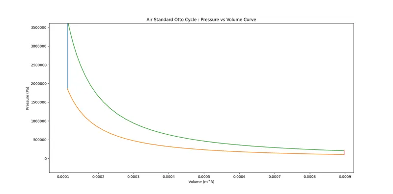
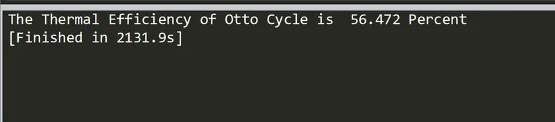
By using the Ideal standard efficiency of the otto cycle we obtain 56.4% for the corresponding compression ratio and the gamma value. This efficiency is the maximum possible theorital efficiency and the practical efficiency is slightly more than half of this efficiency. This efficiency is not possible practically, due to limitations in the environmental condition and the operation pressure and temperature.

References:

[1] Heywood, J. B. (2018). Internal combustion engine fundamentals. McGraw-Hill Education.