Week 5 - Curve fitting

AIM

To make the best possible Curve Fit of the Temperature vs Specific heat with the given practical data using Python.

Objective

To determine best possible curve fit that helps us understand the variation of specific heat and temperature using Python. This best possible fit is used for numerical calculations purpose.

Solution

For determing the best possible fit of the given data we use the library math, matplotlib and scipy.optimize. The math library will be used for performing mathematical operations. The matplotlib library is used for plotting images in python. The scipy.optimize library is used for the solving the unknown parameters in the polynomial equations and to solve the equaitons by determing the constants and therby using this constants to determine the values of temperature as a function of Cp.

Python Code

import numpy as np 
import matplotlib.pyplot as plt 
from scipy.optimize import curve_fit 

def func_linear(t,a,b):
	return a*t+b

def func_quad(t,a,b,c):
	return a*pow(t,2)+b*t+c 

def func_cubic(t,a,b,c,d):
	return a*pow(t,3)+b*pow(t,2)+c*t+d 

def func_poly(t,a,b,c,d,e):
	return a*pow(t,4)+b*pow(t,3)+c*pow(t,2)+d*t+e 

def read_file():
	temperature=[]
	cp=[]
	for line in open('data','r'):
		values=line.split(',')
		temperature.append(float(values[0]))
		cp.append(float(values[1]))
	return[temperature,cp]

# Plots Linear Variation
temperature,cp=read_file()
popt,pcov = curve_fit(func_linear,temperature,cp)
fit_cp=func_linear(np.array(temperature),*popt)

plt.figure()
plt.plot(temperature,cp,color="blue",linewidth=3)
plt.plot(temperature,fit_cp,color="red",linewidth=3)
plt.title('Specific Heat vs Temperature Linear Fit')
plt.legend(['Actual Data','Curve fit'])
plt.xlabel('Temperature[K]')
plt.ylabel('cp')
plt.show()

plt.figure()
# Plots Quadratic Variation
popt,pcov=curve_fit(func_quad,temperature,cp)
fit_cp=func_quad(np.array(temperature),*popt)

plt.plot(temperature,cp,color="blue",linewidth=3)
plt.plot(temperature,fit_cp,color="red",linewidth=3)
plt.title('Specific Heat vs Temperature Quradratic Fit')
plt.legend(['Actual data','Curve fit'])
plt.xlabel('Temperature[K]')
plt.ylabel('cp')
plt.show()

plt.figure()
#Plots Cubic Variation
popt,pcov=curve_fit(func_cubic,temperature,cp)
fit_cp=func_cubic(np.array(temperature),*popt)

plt.plot(temperature,cp,color="blue",linewidth=3)
plt.plot(temperature,fit_cp,color="red",linewidth=3)
plt.title('Specific Heat vs Temperature Cubic Fit')
plt.legend(['Actual data','Curve fit'])
plt.xlabel('Temperature[K]')
plt.ylabel('cp')
plt.show()

plt.figure()
#Plots 4th Order Polynomial Fit Variation
popt,pcov=curve_fit(func_poly,temperature,cp)
fit_cp=func_poly(np.array(temperature),*popt)

plt.plot(temperature,cp,color="blue",linewidth=3)
plt.plot(temperature,fit_cp,color="red",linewidth=3)
plt.title('Specific Heat vs Temperature 4th Order Polynomial Fit')
plt.legend(['Actual data','Curve fit'])
plt.xlabel('Temperature[K]')
plt.ylabel('cp')
plt.show()

Explaination of Python Code

The function func_linear(t,a,b), func_quad(t,a,b,c):, func_cubic(t,a,b,c,d): and func_poly(t,a,b,c,d,e): are used as the variation of linear, quadrature, cubic and 4th order polymial fit for the variation of the Temperature and Cp.

Ex. Quadratic FIT

The Polynomial Equation a*t^2+b*t+c

here : a,b,c - 3 unknowns

The function read_file() is used for taking the first line present in the data file and splits into two array, first array is temperature and the second array is Cp values which is then casting as float values. These values are Appended as array using numpy library.

The function Curve Fit function in scipy modue, the passes the values extracted from the data and is used to determine the values of unknows using the function popt, pcov.

popt is used to calculate the optimal values of the unknowns a,b,c for the Quradratic fit, by minimising the sum of squares of residuals (f(xdata, *popt) - ydata)

pcov is a 2 dimentional Array which estimates the co-variance of the parameter in popt. It can also be used to find the standard deviation errors of popt. The diagonals generally provide the variance of the parameter estimate. And also to compute the single standard deviation of the errors on the parameters we use the equation: perr = np.sqrt(np.diag(pcov)).

once we have a new coefficients (a,b,c), we pass the temperature array as numpy array along with the co-efficients (we are passing *popt).

we have done a curve fit, with the curvefit we will calculate the specific heats again. That is known as fit_cp.

we are plotting two curves in a figue, the temperature vs Cp and temperature vs fit_cp, if the curve fit is perfect then it best represent the actual task. We ploted for linear, quradric, cubic and also for the 4th order Polynomial Equation.

Results and Discussion

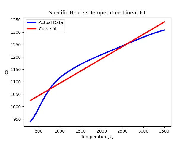
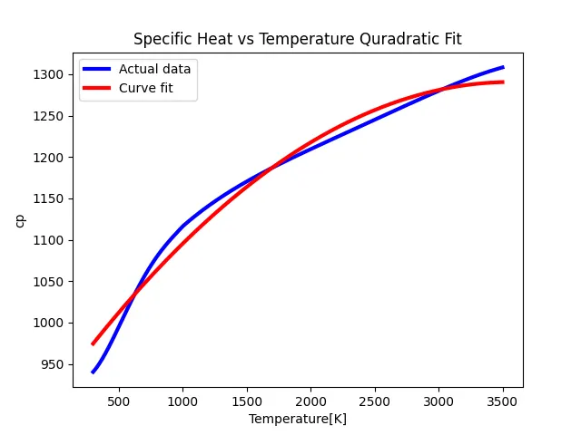
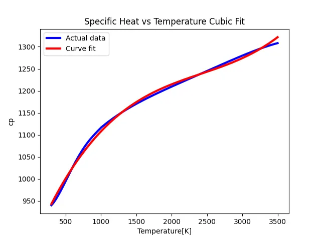
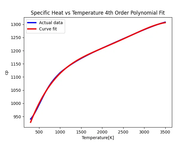
The Below 4 figures represent the variation of Temperature as a variation of Specific Heat. The variation between these graphs are the differences in the fit, linear, qudratic, cubic and the 4th order Polynomicla fit equation. The Red colour line represent the curve fited graph which we obtain after performing curve fit. The blue colour line represent the actual data used for performing curve fit.

Linear FIT

Qudratic FIT

Cubic FIT

4th Order Polynomial FIT

Inference

As the degree of polynomial increases, the fit becomes more accurate. The Actual data is exactly matching with the curve fit curve for the 4th order polynomial. This can clearly found in the graph as shown above.

References

[1] https://docs.scipy.org/doc/scipy/reference/generated/scipy.optimize.curve_fit.html

Used Data:

The practical variation of Temperature vs Cp is obtained from here. https://drive.google.com/file/d/1vWi9Vj3AdQf0gqUK1u9jwS8zg92BHGR0/view