Detailed Analysis of Subsonic-Supersonic & Shockwave Simulation for an Isentropic flow in De-Laval Nozzle
Abstract:
A nozzle is a mechanical device that is designed to control the parametric characteristics of the fluid that exhausts through it. The main purpose of the nozzle is to increase the velocity of fluid flow by dropping the pressure. Depending on the application there are various types of nozzles out of which the De-Laval nozzle (Convergent-Divergent nozzle) is mainly used for supersonic applications. In this report, we are going to analyse the traditional Isentropic Subsonic-Supersonic, & Shockwave simulation for a Quasi 1-D flow in a convergent-divergent nozzle. This report provides the basic theoretical concepts and methodology used for the analysis of the De-Laval nozzle. It also includes both Analytical and Numerical results of the De-Laval nozzle and a comparison of both the results against each other. Analytical results are calculated by using standard mathematical formulas used to solve C-D Nozzle problems, which are taken from a textbook called “Computational Fluid Dynamics” by JOHN D. ANDERSON.JR Chapter-7 Quasi 1-D Nozzle flow. Numerical analysis was done by using a commercial CFD package called ANSYS FLUENT. The variation of flow parameters like Pressure, Temperature, Velocity, and Density has been monitored & visualized.
Keywords: De-Laval nozzle, CFD = Computational Fluid dynamics, ANSYS Fluent.
Symbols:
- `P`=Pressure (`Pa`)
- `T`=Temperature (`K`)
- `V`=Velocity (`m/s`)
- `C`= Velocity of sound (`m/s`)
- `g`=Gravitational acceleration (`m/s^2` )
- `dotm` = Mass flow rate (kg/s)
- `rho`= Density (`(kg)/(m^3)` )
- `A`=Cross sectional area (`m^2`)
- `C_p`=Specific heat at constant pressure (`J/(kg-K)`)
- `H` = Enthalpy (`J`)
- `gamma`= Isentropic index
- `R`= Specific gas constant (`J/(kg-K)`)
- `M_a`= `V/C`Mach number
1.0 Literature Review on Fluid Flow through a C-D Nozzle
1.1 INTRODUCTION
- Nozzle is a device used to alter and control the mass flow rate, velocity, direction of flow, and pressure ratio. The design of the nozzle is considered to be like a pipe with varying cross-sectional areas throughout the length. It has the capacity to convert the thermo-chemical energy generated in the combustion chamber into useful kinetic energy. The nozzle converts the high pressure, low velocity, high-temperature gas in the combustion chamber into high-velocity gas of lower pressure and low-temperature gas. Depending on the application we have different nozzle shapes. For high-speed applications like supersonic aircraft, missiles, and rocket engines we use a Convergent divergent nozzle.
- In the present day, there is a huge development in Aerospace Engineering for various prospects. Extensive research is being carried out in the fields like civil and defence prospects. The computational techniques are being more popular for getting better results, which are close to experimental techniques. Flow-through a convergent-divergent nozzle is one of the benchmark problems used for modelling the compressible flow using computational fluid dynamics. In this paper, CFD analysis of a convergent-divergent rocket nozzle is done obtaining results at various positions of the nozzle.
1.2 LITERATURE REVIEW
- “Concepts and CFD Analysis of De-Laval Nozzle” by Dr. D.Y Patil Institute of Engineering and Technology, Pune, India. In this paper, a CFD analysis of the De-Laval Nozzle has been done. He explained all the basic concepts of De Laval nozzle along with providing the CFD of each and every case. Comparison is done based on theoretical and CFD values.
- “Modelling and simulation of Supersonic nozzle using computational fluid dynamics, by Venkatesh V and C Jayapal Reddy. In this paper theoretical and CFD analysis of various types of nozzles is given. Also thrust conditions and design parameters are discussed in this nozzle.
- Nazar Muneam Mahmood simulated the steady flow of a gas through a C-D nozzle which has a varying cross-sectional area and showed that the nature of the flow can be explained by considering how the flow and its characteristics in the nozzle change as the backpressure decreases.
1.3 Rocket or Air Breathing Nozzle
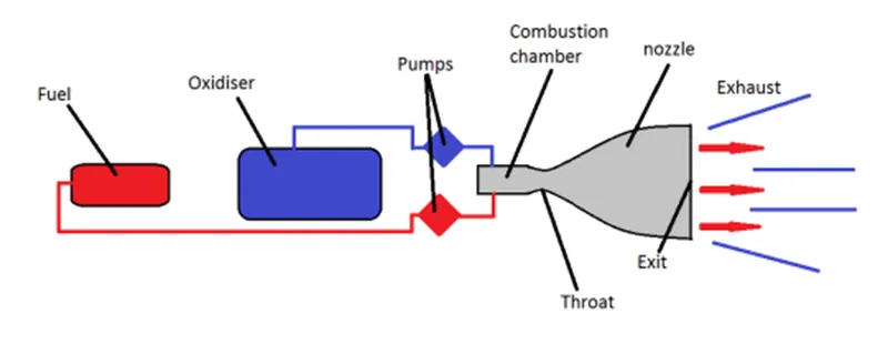
Thrust Operation
- The ultimate purpose of a nozzle is to expand a gas as efficiently as possible to maximize the exit velocity. This will increase the thrust produced. The thrust produced is given by the equation.
- `F = ṁ V_e + (P_e − P_0)A_e`
- A rocket generally does not travel through a single altitude, thus while designing a path over which a rocket is to travel is considered so that the expansion ratio that maximizes the performance is selected. Other factors like nozzle weight, length, manufacturability, heat transfer, and aerodynamic characteristic are also considered while designing thus altering the shape of the nozzle.
1.4 DE LAVAL NOZZLE:
- De-Laval nozzle or Converging Diverging Nozzle is the most widely used type of nozzle to achieve supersonic velocities. It was first developed by a Swedish engineer named Carl Gustaf De Laval in the year 1888. The design of the C-D nozzle is like a tube that is pinched in the middle, making a carefully balanced, asymmetric hourglass shape. It is used to accelerate a compressible fluid to supersonic speeds in the axial (thrust) direction, by converting the thermal energy of the flow into kinetic energy. It is widely used in supersonic jet engines and steam turbines. They also have certain applications in the jet streams within astrophysics.
- C-D nozzle is composed of three sections: a converging section, a throat, and a diverging section.
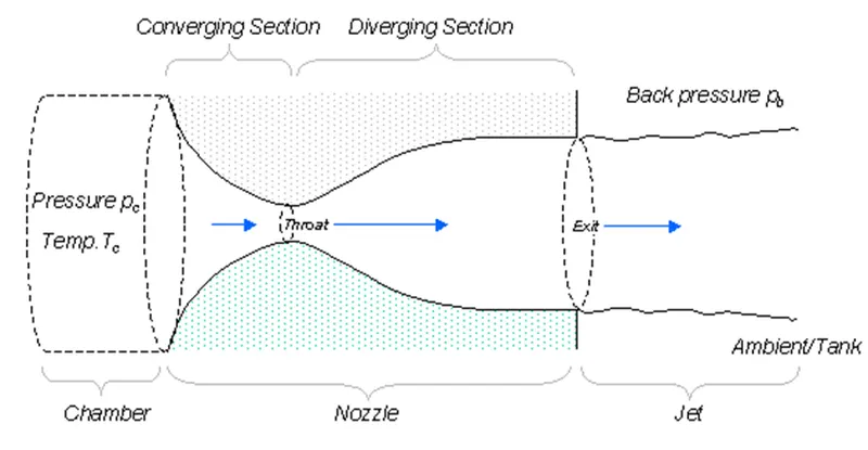
1.4.1 Expansion Ratio
- The expansion ratio of the nozzle is the ratio of the exit area to the throat area.
`ε = A_e /A^∗`
1.4.2 Isentropic Flow
An isentropic flow is the ideal type of flow as it is both adiabatic no heat addition and inviscid. This assumption may be justified by the following.
- Heat transfer effects between the flow and the nozzle walls are minimal due to the short-run times of the high-speed flow.
- The Reynolds number of the core is much higher than the Reynolds number near the nozzle walls.
- Due to the characteristic length of the nozzle core being greater.
1.4.3Choked flow
- Choked flow is a compressible flow effect. For a fixed upstream pressure and temperature, Fluid always flows from a high-pressure region to a low-pressure region, depending on the downstream pressure mass flow rate varies for a fixed geometry. At a particular downstream pressure, the mass flow rate reaches the maximum and there is no further decrease in the mass flow for a further decrease in the downstream pressure environment.
1.5 Flow in Different Sections
- Flow in Converging section:
- Flow exits from a source or reservoir enter into the converging section of the nozzle at this moment flow is in subsonic condition (M<1). The design of the converging section is just like a conical tube with decreasing cross-section. Once the flow entered the converging section of the nozzle, the flow accelerates due to decreasing area. This is justified via the conservation of mass flow rate. The flow continues downstream to the throat, where the cross-sectional area is the smallest.
- Flow Regimes at Throat:
- For a perfectly designed nozzle flow velocity at the throat is sonic (M=1). Flow at the throat is called chocked flow. In order for the nozzle to reach sonic conditions at the throat, the inlet cross-sectional area to throat area ratio must be a certain value Additionally, the inlet-to-exit pressure ratio must be a certain value that corresponds to the free stream Mach number.
- Flow in Diverging section:
- Finally, the flow enters the diverging section where it becomes supersonic (M>1) and accelerates to the design Mach number. The design of the diverging section is just like a conical tube with an increasing cross-section. Once the flow entered the diverging section of the nozzle, the flow accelerates due to flow expansion along the length of the tube. Due to the supersonic velocities in the diverging section sound wave will not propagate backward through. Sometimes, the fluid may decelerate in the diverging section instead of accelerating if the backpressure is not in the range creating subsonic flow at the outlet. Thus, the state of nozzle flow is determined by the Overall Pressure Ratio
- `O.P. R = P_b /P_0` ---------------(1)
- Finally, the flow enters the diverging section where it becomes supersonic (M>1) and accelerates to the design Mach number. The design of the diverging section is just like a conical tube with an increasing cross-section. Once the flow entered the diverging section of the nozzle, the flow accelerates due to flow expansion along the length of the tube. Due to the supersonic velocities in the diverging section sound wave will not propagate backward through. Sometimes, the fluid may decelerate in the diverging section instead of accelerating if the backpressure is not in the range creating subsonic flow at the outlet. Thus, the state of nozzle flow is determined by the Overall Pressure Ratio
1.6 Operation C-D nozzle under varying back pressures:
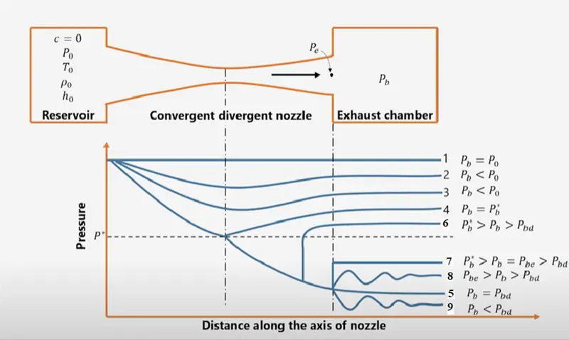
- Here we have a converging-diverging nozzle a reservoir is attached to the entry and an exhaust chamber is attached to the exit. Inside the reservoir properties are stagnation properties and in the exhaust, the chamber is maintained at back pressure P_b, P_b can be adjusted by a valve, at the exit of C-D nozzle we have pressure called P_e.
No Flow
- 1. No Flow (P_b = P_o):
- Initially, stagnation pressure and exhaust chamber are maintained at constant pressure. hence there won't be any flow taking place the pressure value throughout the nozzle will be the same.
Subsonic flow
- 2. Subsonic flow (P_b < P_o):
- There is a slight decrease in the backpressure to P_2. Flow takes place through the nozzle. Initially, the flow will be considered as incompressible and subsonic through convergent path flow accelerates & pressure decreases reaches to a minimum at the throat and in the diverging part flow is decelerated and pressure increased.
- 3. Subsonic flow (P_b << P_o):
- Further decrease in the backpressure to P_3. flow is the Same as above with increased mass flowrate.
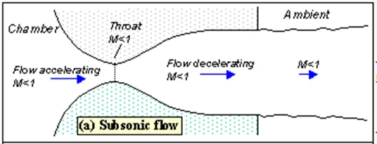
Sonic flow:
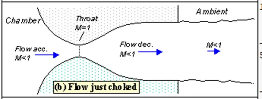
- 4. Flow just Chocked (P_b=P_b^*):
- There is a further decrease in the backpressure to P_4. We eventually get to the situation where the flow pattern is exactly the same as in subsonic flow, except that the flow speed at the throat has just reached Mach number of unity. Correspondingly flow properties at this stage are called critical properties denoted by an asterisk to denote chocked flow properties. Flow through the nozzle is now choked since further reductions in the backpressure can't move the point of M=1 away from the throat.
Supersonic Flow:
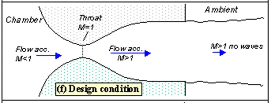
- 5. Design Condition (P_b=P_(bd)):
- Further decrease in the back pressure P_5 to the design pressure P_(bd). where we can able to generate a smooth supersonic flow at the exit. In the converging part, flow accelerates at the subsonic and reaches a sonic speed at the throat, and in the diverging part, flow accelerates with supersonic speed.
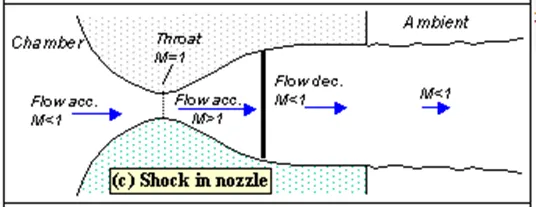
- 6. Shock in the nozzle (P_b^*>P_b>P_(bd)):
- If we maintain the pressure in between critical pressure P^* and design pressure P_(bd). A normal shock is generated somewhere in the diverging section. The position of the shock is anywhere between diverging sections. The shock wave produces instantaneous deceleration of the flow from supersonic to subsonic speed. This subsonic flow then decelerates further and exhausts from the subsonic jet. In this regime, if you lower or raise the back pressure you increase or decrease the length of supersonic flow length in the diverging section before the shock wave.
- If we maintain the pressure in between critical pressure P^* and design pressure P_(bd). A normal shock is generated somewhere in the diverging section. The position of the shock is anywhere between diverging sections. The shock wave produces instantaneous deceleration of the flow from supersonic to subsonic speed. This subsonic flow then decelerates further and exhausts from the subsonic jet. In this regime, if you lower or raise the back pressure you increase or decrease the length of supersonic flow length in the diverging section before the shock wave.
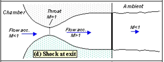
- 7. Shock at exit (P_b^* > P_b=P_(be)>P_(bd)):
- If we lower the backpressure to P_7 near to the design pressure until the shock is sitting at the nozzle exit. In this case, we have a very long region of acceleration. Flow speed just before the shock will be supersonic however, after the shock the flow in the jet will still be subsonic.
- If we lower the backpressure to P_7 near to the design pressure until the shock is sitting at the nozzle exit. In this case, we have a very long region of acceleration. Flow speed just before the shock will be supersonic however, after the shock the flow in the jet will still be subsonic.
- 8. Overexpanded (P_(be)>P_b>P_(bd)):
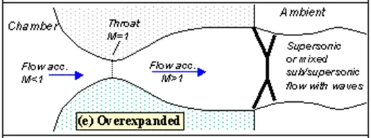
- If we reduce pressure further to P_8 >P_(bd) causes the shock to bend out into the exhaust chamber and a complex pattern of shocks and reflections is set up at the exit which will now involve a mixture of subsonic and supersonic flow, shock is no longer perpendicular to the flow, therefore these shocks are called oblique shocks at the outlet.
- If we reduce pressure further to P_8 >P_(bd) causes the shock to bend out into the exhaust chamber and a complex pattern of shocks and reflections is set up at the exit which will now involve a mixture of subsonic and supersonic flow, shock is no longer perpendicular to the flow, therefore these shocks are called oblique shocks at the outlet.
- 9. Under expanded (P_b<P_(bd)):
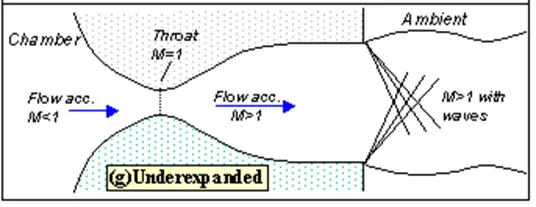
- Finally, if we lower the exhaust chamber back pressure below the design back pressure to P_9. There will create a new imbalance between the exit and back pressures apart from this imbalance expansion curve is similar to the design pressure expansion curve. There won’t be any effect throughout the nozzle.
- Finally, if we lower the exhaust chamber back pressure below the design back pressure to P_9. There will create a new imbalance between the exit and back pressures apart from this imbalance expansion curve is similar to the design pressure expansion curve. There won’t be any effect throughout the nozzle.
1.6.1 Pressure distribution in the nozzle
- Flow inside the nozzle accelerates by dropping the pressure.
- There is an instantaneous rise in the pressure across the shock.
- The pressure throughout the nozzle is always the same as the ambient unless the jet is supersonic and there are shocks or expansion waves in the jet to produce pressure differences.
- The pressure falls across an expansion wave.
1.7 Expansion Analysis of Nozzle
- Based on the exit and atmospheric pressure we have four cases to be taken into consideration
- `P_e` = Exit pressure,
- `P_(atm)` = atmospheric pressure
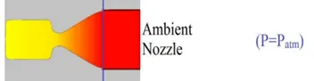
- Case 1 : `P_e = P_(amb)`: Ambient Nozzle:
- In this case, Flow is perfectly expanded, and thus it provides maximum efficiency.
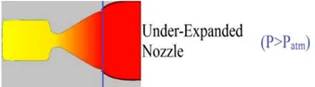
- Case 2 : `P_e > P_(amb)`: Under Expanded Nozzle:
- In this case, flow continues to expand outwards after leaving the nozzle. This expansion does not contribute to the thrust production as it does not exert any pressure on the nozzle wall. Thus, it reduces efficiency. The nozzle should have been longer to capture this expansion and convert it into thrust.
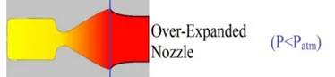
- Case 3:`P_e: Over Expanded nozzle:
- In this case, Exit pressure is less than the ambient atmospheric pressure. Thus, the external pressure pinches the flow into the nozzle. This reduces the efficiency as the extra nozzle wall is wasted as it does not generate additional thrust. Thus, the nozzle should be shorter to eliminate the unnecessary wall.
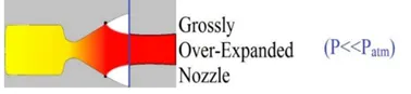
- Case 4 : `P_e < < P_(amb)`: Grossly Over-Expanded Nozzle:
- This ambient pressure is too large compared to the exit pressure. Hence it is given the name grossly expanded nozzle.
Some typical values of exhaust gas velocity `V_e` for rocket engines burning various propellants using the De-Laval nozzle are:
- 1700 to 2900 m/s (3800 to 6500 mph) for liquid monopropellants.
- 2900 to 4500 m/s (6500 to 10,100 mph) for liquid bipropellants.
- 2100 to 3200 m/s (4700 to 7200 mph) for solid propellants.
1.8.1 Reduced-Order Model
A reduced-order model is used as a preliminary design tool to give a prediction of the nozzle’s performance. A quasi-one-dimensional Matlab program was written to provide a visual representation of the flow conditions. The Matlab program intakes the nozzle geometry and determines the Mach number, temperature ratio, pressure ratio, and any shocks that may occur based on flow conditions. The values are presented graphically while the flow passes through the nozzle. Regardless, this reduced-order model is not useful for the design of the nozzle’s contour to ensure a shock-free flow.
1.8.2 Quasi-One-Dimensional Flow
A quasi-one-dimensional flow (quasi-1D flow) is a flow in which the flow parameters only vary in one direction. A quasi-1D flow analysis yields a top-level design for a nozzle. Mainly, this analysis calculates rough pressure ratios and expansion ratios for the design Mach number.
------------------------------------------------------------------------------------------------------------------------------------
2.0 Calculation theory of Convergent Divergent Nozzle.
2.1 Problem: Subsonic - Supersonic Isentropic flow.
- Let us consider the steady, isentropic flow through a convergent-divergent nozzle. The flow from the inlet to the nozzle comes from a reservoir where the pressure and temperature are denoted by `P_o`, and `T_o` respectively. The cross-sectional area of the reservoir is large (theoretically, `A=>infty`), and hence the velocity is very small (`V=>0`). Thus, `P_o` and `T_o` are the stagnation values. Depending on the pressure ratio the flow expands isentropically to subsonic or supersonic speeds at the nozzle exit, where the exit pressure, temperature, velocity, and Mach number are denoted by `P_e, T_e, V_e`and `M_e`, respectively. The flow is locally subsonic in the convergent section of the nozzle, sonic at the throat (minimum area), and subsonic/supersonic at the divergent section. The sonic flow (`M = 1`) at the throat means that the local velocity at this location is equal to the local speed of sound. Using an asterisk to denote sonic flow values, we have at the throat `V=V^**= a^**`. Similarly, the sonic flow values of pressure and temperature are denoted by `P^**` and `T^**`, respectively. The area of the sonic throat is denoted by `A^**`. We assume that at a given section, where the cross-sectional area is A, the flow properties are uniform across that section. Hence, although the area of the nozzle changes as a function of distance along the nozzle, x, and therefore in reality the flow field is two-dimensional (the flow varies in the two-dimensional XY space), we make the assumption that the flow properties vary only with x; this is tantamount to assuming uniform flow properties across any given cross-section. Such flow is defined as quasi-one-dimensional flow.
- The governing continuity, momentum, and energy equations for this quasi-one-dimensional, steady, isentropic flow can be expressed, respectively, as
-
- Continuity: `rho_1V_1A_1=rho_2V_2A_2`-------------------------(2)
- Momentum: `P_1A_1+rho_1V_1^2A_1+int_(A_1)^(A_2)PdA =P_2A_2+rho_2V_2^2A_2` -------(3)
- Energy: `h_1+V_1^2/2=h_2+V_2^2/2` -------------------------(4)
- where subscripts 1 and 2 denote different locations along with the nozzle. In addition, we have the perfect gas equation of state,
-
- `P = rhoRT` -------------------------(5)
- as well as the relation for a calorically perfect gas,
-
- `h = C_pT` -------------------------(6)
- The above equations can be solved analytically for the flow through the nozzle.
2.2.1 Stagnation Properties:
- During a stagnation process, the kinetic energy of the fluid is converted to enthalpy which results in an increase in fluid temperature and pressure. The properties of the fluid in a stagnation state are called stagnation properties. `T_0` is stagnation temperature and `P_0` is stagnation pressure. `T_0` is the temperature an ideal gas attains when it is brought to rest adiabatically.`rho_o` is stagnation density.
-
- `T_0=T+V^2/(2C_p)`-------------------------(7)
- `P_0`is pressure it attains when fluid is brought to rest adiabatically.
-
- `P_0/P= (T_0/T)^(gamma/(gamma-1))`-------------------------(8)
- `rho_o/rho= (T_0/T)^(1/(gamma-1))`-------------------------(9)
- Note: `T, P, rho` are inlet conditions
2.2.2 Density for an ideal gas:
- `rho = (M_w **P)/(R**T)` `(Kg)/m^3` ------------------------(10)
- `M_w ` = Molecular weight in `(Kg)/(mol)`
- `R` = Gas Constant `8.31446 J/(mol-K)` `J = Pa**m^3`
2.3 Convergent Divergent nozzle equations
- The Mach number variation through the nozzle is governed exclusively by the area ratio `A/A^**` through the relation. The Mach number variation is given by:
-
- `A/A^**=1/M_a[(2/(gamma+1))(1+((gamma-1)/2)M_a^2)]^((gamma+1)/(2(gamma-1)))`------------------------(11)
- `A^**`is the area of the nozzle at the throat.
- where `gamma` = ratio of specific heats = `C_p/C_v`. For air at standard conditions, `gamma = 1.4`. For a nozzle where A is specified as a function of `x`, hence `A/A^**` is known as a function of x, `A/A^**` equation allows the (implicit) calculation of M as a function of x. The variation of pressure, density, and temperature as a function of Mach number.
- `A/A^**=1/M_a[(2/(gamma+1))(1+((gamma-1)/2)M_a^2)]^((gamma+1)/(2(gamma-1)))`------------------------(11)
- The pressure variation is given by,
- `P_0/P=[1+((gamma-1)/2)M_a^2]^((gamma)/(gamma-1))`------------------------(12)
- The temperature variation is given by,
- `T_0/T=[1+((gamma-1)/2)M_a^2]`------------------------(13)
- The density variation is given by,
-
- `rho_0/rho=[1+((gamma-1)/2)M_a^2]^(1/(gamma-1))`------------------------(14)
- The mass flow rate is given by,
- `dotm= PAM_asqrt(gamma/(RT))`------------------------(15)
In this case, the force exerted on the gas to accelerate it through the nozzle is supplied by the pressure ratio across the nozzle, `p_o/p_e`. For a nozzle with a specified area ratio `A_e/A^**`, the pressure ratio is required to establish the subsonic-supersonic isentropic flow.
2.4 Shockwave :
- Shock is an abrupt discontinuity in the flow field and it occurs inflows when the local flow speed exceeds the local sound speed. More specifically, it is a flow whose Mach number exceeds 1.
- Shock is also some kind of expansion wave that happens only in the supersonic flow. When shock occurs in the flow there will be abrupt changes in fluid properties occur in a very thin section. Before the shock happens, flow is in supersonic condition due to the shock there by a sudden increase in the pressure and flow becomes subsonic.
- A shock wave is a type of propagating disturbance that moves faster than the local speed of sound in the medium. Like an ordinary wave, a shock wave carries energy and can propagate through a medium but is characterized by an abrupt, nearly discontinuous, change in pressure, temperature, and density of the medium.
- When an object is moving in a flow field the object sends out disturbances that propagate at the speed of sound and adjusts the remaining flow field accordingly. However, if the object itself happens to travel at speed greater than sound, then the disturbances created by the object would not have traveled and communicated to the rest of the flow field and this results in an abrupt change of property, which is termed as a shock in gas dynamics terminology.
- Shocks are characterized by discontinuous changes in flow properties such as velocity, pressure, temperature, etc. Typically, shock thickness is of a few mean free paths(of the order of 10−8 m). Shocks are irreversible occurrences in supersonic flows.
2.4.1 Normal shocks:
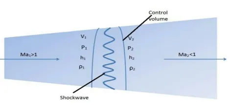
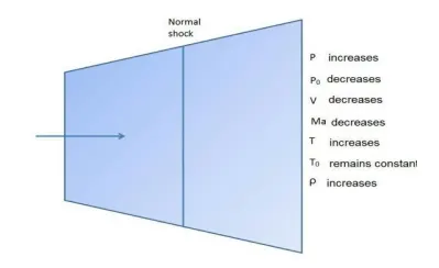
- Normal shocks generally occur in a plane normal (90* perpendicular) to the direction of the shock flow medium. Across a normal shock, the total pressure suddenly decreases, The supersonic flow before the shock becomes subsonic immediately after the shock. Therefore, the flow must changes from supersonic to subsonic if a shockwave is to occur. The larger the Mach number before the shock, the stronger the shock will be. In the limiting case of `M_a=1`, the shock wave simply becomes a sound wave.
- According to the conservation of energy principle, the stagnation enthalpy remains constant across the shock; `h_01=h_02`. The stagnation temperature is also constant `T_01=T_02`. The stagnation pressure decreases across the shock, because of irreversibility, while the ordinary temperature rises drastically because of the conversion of kinetic energy into enthalpy due to a large drop in fluid velocity.
- The equations between various properties before and after the shock for an ideal gas are as follows: The temperature ratio is given by
- `T_2/T_1=[1+((gamma-1)/2)M_(a1)^2]/[1+((gamma-1)/2)M_(a2)^2]`------------------------(16)
- Fanno flow is the adiabatic flow through a constant area duct where the effect of friction is considered. Compressibility effects often come into consideration, although the Fanno flow model certainly also applies to incompressible flow.
- The pressure ratio for the Fanno line is given by,
- `P_2/P_1=(M_(a1)sqrt[1+((gamma-1)/2)M_(a1)^2])/(M_(a2)sqrt[1+((gamma-1)/2)M_(a2)^2]` ------------------------(17)
- Rayleigh flow refers to frictionless, non-adiabatic flow through a constant area duct where the effect of heat addition or rejection is considered. Compressibility effects often come into consideration, although the Rayleigh flow model certainly also applies to incompressible flow.
- The pressure ratio for the Rayleigh line is given by,
- `P_2/P_1=(1+gammaM_(a1)^2)/(1+gammaM_(a2)^2)`------------------------(18)
- The Mach number relation for before and after shockwave is given by,
- `M_(a2)^2=[M_(a1)^2+(2/(gamma-1))]/[2M_(a1)^2(gamma/(gamma-1))-1]` ------------------------(19)
2.4.2 Oblique Shocks
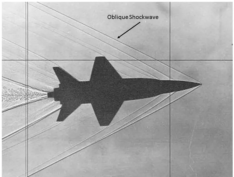
- When the flow field is still attached to the body, the shock wave which is deviating (inclined) at some arbitrary angle from the flow direction is termed oblique shock. Oblique shock is generally generated at the nose of the nozzle during downstream flow. Oblique shock generally occurs when the supersonic flow is encountered at a corner that effectively turns the flow into itself and compresses it. It can be converted to a normal shock by a Galilean transformation.
2.5 Prandtl–Meyer expansion fan:
- Prandtl–Meyer expansion fan, a two-dimensional simple wave, is a centered expansion process that occurs when a supersonic flow turns around a convex corner. The fan consists of an infinite number of Mach waves, diverging from a sharp corner. When a flow turns around a smooth and circular corner, these waves can be extended backward to meet at a point.
- Each wave in the expansion fan turns the flow gradually (in small steps). It is physically impossible for the flow to turn through a single "shock" wave because this would violate the second law of thermodynamics. Across the expansion fan, the flow accelerates (velocity increases) and the Mach number increases, while the static pressure, temperature, and density decrease. Since the process is isentropic, the stagnation properties (e.g. the total pressure and total temperature) remain constant across the fan.
------------------------------------------------------------------------------------------------------------------------------------
3.0 Shape and Analytical Calculation
3.1 The shape of the Convergent-Divergent nozzle:
-
- The basic shape of the nozzle is taken from a journal called "CONCEPTS AND CFD ANALYSIS OF DE-LAVAL NOZZLE" by Malay S Patel, Sulochan D Mane, and Manikant Raman
-
Parameter Dimension The total length of the nozzle 0.840 (m) Inlet diameter 0.280 (m) Outlet diameter 0.336 (m) Throat diameter 0.210 (m) Convergence angle 30.55 (deg) Divergence angle 54.532 (deg)
-
- The detailed shape of the nozzle shape curvature was taken from a website called https://cfd.ninja/
-
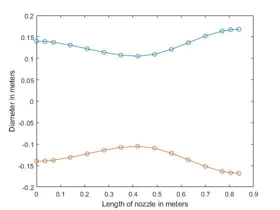
S.No X (m) Y (m) 1 0.000 0.14000 2 0.035 0.13930 3 0.070 0.13755 4 0.140 0.13090 5 0.210 0.12250 6 0.280 0.11410 7 0.350 0.10752 8 0.420 0.10500 9 0.490 0.10948 10 0.560 0.12124 11 0.630 0.13664 12 0.700 0.15204 13 0.770 0.16366 14 0.805 0.16688 15 0.840 0.16800
-
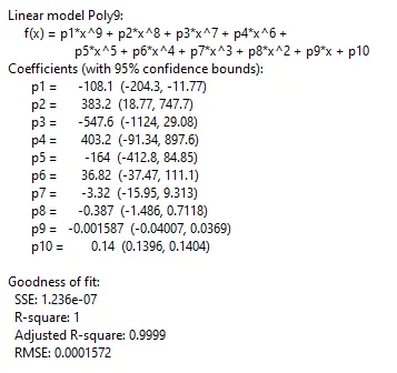
- 9th order non-linear equation satisfies the above co-ordinates
- Writing co-ordinate text file
- Writing MATLAB Code to create a Nozzle_shape_coordinate.text file. So that Ansys Solidmodeller can read the file and plot the points and curve.
-
% Convergent Divergent Nozzle Shape clear all; close all; clc %% Nozzle geometry X = [0.00, 0.035, 0.07, 0.14, 0.21, 0.28, 0.35, 0.42, 0.49, 0.56, 0.63, 0.70, 0.77, 0.805, 0.84]; Radius = [0.14, 0.1393, 0.13755, 0.1309, 0.1225, 0.1141, 0.10752, 0.105, 0.10948, 0.12124, 0.13664, 0.15204, 0.16366, 0.16688, 0.168]; %%creating nozzle co-ordinate text file curve = fopen('Nozzle_shape_coordinates.txt','w'); fprintf(curve,'polyline=truen'); % polyline=true command tells design modeller to draw a polyline through the below co-ordinates for i = 1:length(X) fprintf(curve, '1 %10.3d %10.5d n', X(i), Radius(i)); end fclose(curve); %% Figures figure(1) plot(X,Radius,'-o','MarkerIndices',1:1:length(Radius)) hold on plot(X,-Radius,'-o','MarkerIndices',1:1:length(Radius)) xlabel("Length of nozzle in meters") ylabel("Diameter in meters") figure(2) plot(X(1:8),Radius(1:8),'b',X(1:8),-Radius(1:8),'b') hold on plot(X(8:15),Radius(8:15),'r',X(8:15),-Radius(8:15),'r') hold off xlabel("Length of nozzle in meters") ylabel("Diameter in meters") - Nozzle_shape_coordinates.txt
- The "polyline=true" command tells the modeler to draw a polyline through the below coordinates mentioned below.
-
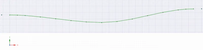
polyline=true 1 000 1.40000e-01 1 3.500e-02 1.39300e-01 1 7.000e-02 1.37550e-01 1 1.400e-01 1.30900e-01 1 2.100e-01 1.22500e-01 1 2.800e-01 1.14100e-01 1 3.500e-01 1.07520e-01 1 4.200e-01 1.05000e-01 1 4.900e-01 1.09480e-01 1 5.600e-01 1.21240e-01 1 6.300e-01 1.36640e-01 1 7.000e-01 1.52040e-01 1 7.700e-01 1.63660e-01 1 8.050e-01 1.66880e-01 1 8.400e-01 1.68000e-01 - Figure (1) Profile with co-ordinate points
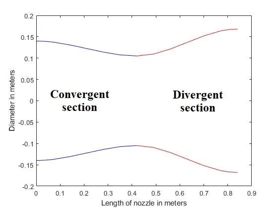
- Figure (2) Convergent Divergent section
- The basic shape of the nozzle is taken from a journal called "CONCEPTS AND CFD ANALYSIS OF DE-LAVAL NOZZLE" by Malay S Patel, Sulochan D Mane, and Manikant Raman
3.2 Analytical Calculation Procedure:
- Analytical results are calculated based on equations 11-14. These equations are coded in MATLAB to automate the calculation. Since equation 11 Area-Mach number relation is a non-linear 2nd order equation that can be solved by using "fsolve" inbuild command in MATLAB but we are using the Newton-Raphson method for better accuracy.
- For Supersonic condition:
- Rewriting equation 11 Area-Mach number relation in function form :
- `A/A^**=1/M_a[(2/(gamma+1))(1+((gamma-1)/2)M_a^2)]^((gamma+1)/(2(gamma-1)))`
- `A = 2/(gamma+1)`
- `B = (gamma-1)/2`
- `C=(gamma+1)/(2(gamma-1))`
- `A_(ratio)=A/A^**`
- `f(M)=A _(ratio) **M − ( A ⋅ (1+ B M^ 2 ) ) C=0`------------------------(20)
- `f'(M)=d/(d M) [ A_(ratio)** M − ( A ** ( B** M^ 2 + 1 ) ) ^C ]`
- `=A_(ratio) ** d/(dM) [ M ] − d/(dM) [ ( A ** ( B** M^2 + 1 ) )^C ]`
- `=A_(ratio) ** 1 − C ** ( A ** ( B** M^ 2 + 1 ) )^(C-1)** d/ (d M) [ A ** ( B** M^2 + 1 ) ]`
- `=A_(ratio) − C ** ( A **( B**M ^2 + 1 ) ) ^(C − 1)** A ** ( d/(d M) [ B** M^ 2 ] + d/(dM) [ 1 ] )`
- `=A_(ratio) − C**A ** ( A ** ( B** M^2 + 1 ) )^( C − 1) **B ** 2M`
- `=A_(ratio) − C**A ** ( cancel(A) ** ( B** M^2 + 1 ) )^ C/(cancel(A) ** ( B** M^2 + 1 ))**B ** 2M)`
- `f'(M)=A_(ratio) − 2**B**C**M(A** ( B** M^2 + 1 )) ^ C/(( B** M^2 + 1 ))=0` ------------------------(21)
- Function code to calculate `f(M)` and `f'(M)` equation 20 & 21
-
%%Function code to calculate `f(M)` and `f'(M)`
function [f, f_prime] = area_mach_fun(Area_ratio,M_guess)
    gama = 1.4; % adiabatic index
    A = 2/(gama+1);
    B = (gama-1)/2;
    C = (gama+1)/(2*(gama-1));
    %% `f(M)`
    f = Area_ratio*M_guess - (A*(1+B*M_guess^2))^C;
    %% `f'(M)
    f_prime = Area_ratio - 2*A*B*C*M_guess*(A*(1+B*M_guess^2))^(C-1);
end
-
- Function code to calculate Pressure, Temperature, Velocity, Density using equations 12,13 & 14
-
%% Function code to calculate Pressure, Temperature, Velocity, Density
function [Pressure, Temperature, Velocity, Density] = pressure_temperature_velocity(Mach_N,P_i,T_i,Rho_i,gamma,Mol_mass,R)
    a = (gamma-1)/2;
    b =  gamma/(gamma-1);
    c =  1/(gamma-1);

    Pressure = P_i/((1+a*Mach_N^2)^b);                  % Pa
    Temperature = T_i/(1+a*Mach_N^2);                   % K
    sound_speed = sqrt((gamma*R*Temperature)/Mol_mass); % m/s
    Velocity = Mach_N*sound_speed;                      % m/s
    Density = Rho_i/((1+a*Mach_N^2)^c);                 % Kg/M^3

end
-
- Main code to calculate Analytical Results at various positions on the X:
-
% Convergent Divergent Nozzle Analytical results
clear all; close all; clc

%% Nozzle geometry
X = [0.00, 0.035, 0.07, 0.14, 0.21, 0.28, 0.35, 0.42, 0.49, 0.56, 0.63, 0.70, 0.77, 0.805, 0.84];
Radius = [0.14, 0.1393, 0.13755, 0.1309, 0.1225, 0.1141, 0.10752, 0.105, 0.10948, 0.12124, 0.13664, 0.15204, 0.16366, 0.16688, 0.168];

%% Entry properties
P_i    = 2000000;       % Inlet Pressure Pa  2 bar
T_i    = 300;          % Inlet Temeperatue K
V      = 175;          % Inlet Velocity m/s

%% Ideal Gas properties & Density calculation
C_p    = 1006.43;           % Specific heat j/kg-K
gamma  = 1.4;               % Gas index Cp/Cv
R = 8.314463;               %Universal gas constant J/(mol-K)
Mol_mass = 0.028966;        % Molecular weight Kg/mole

% Density of air Kg/m^3
Rho_i = (Mol_mass*P_i)/(R*T_i);

%% Area & Area Ratio calculation over a length of domain
% For an 2-D section Area = Diameter
A_At = (2*Radius)/(2*min(Radius));      % Area ratio A/At = A/A*

%%  Solving non linear Area-Mach number equation using Newton raphson method A_At*x-(A*(1+B*x^2))^C
A = 2/(gamma+1);
B = (gamma-1)/2;
C = (gamma+1)/(2*(gamma-1));

Mach_N      = [];
iterations = [];
for i = 1:length(A_At)

    alpha   = 0.2;          % Under relaxation factor
    tol = 1e-6;             % Error tolerance
    itr = 0;
    if i<=length(A_At)/2
        M_guess = 0.001;
        M_old = 100;
        while (abs(M_guess-M_old) >= tol)
            [f, f_prime] = area_mach_fun(A_At(i),M_guess);
            M_old = M_guess;
            M_guess = M_guess - alpha*(f/f_prime);
            itr = itr + 1;
        end
    else
        M_guess = 10;
        M_old = 100;
        while (abs(M_guess-M_old) >= tol)
            [f, f_prime] = area_mach_fun(A_At(i),M_guess);
            M_old = M_guess;
            M_guess = M_guess - alpha*(f/f_prime);
            itr = itr + 1;
        end
    end

    Mach_N(i) = M_guess;
    iterations(i) = itr;
end

%% Flow parameters calculation
Pressure = [];
Temperature = [];
Velocity  = [];
Density   = [];
results = fopen('Results.txt','w');   % writing text file for Analytical results
fprintf(results,"Analytical resultsn")
fprintf(results,'%5s %10s %10s %15s %10s %10s %10sn','X  ','A_At','Mach_N','Pressure','Temperature','Velocity','Density');
for i = 1:length(Mach_N)
    %For analytical calculation Stagnation properties are equal to Inlet Properties
    [Pressure(i), Temperature(i), Velocity(i), Density(i)] = pressure_temperature_velocity(Mach_N(i),P_i,T_i,Rho_i,gamma,Mol_mass,R);
    fprintf(results,'%5.3f %10.5f %10.5f %15.5f %10.5f %10.5f %10.5fn',X(i), A_At(i), Mach_N(i),Pressure(i),Temperature(i),Velocity(i),Density(i));
end
fclose(results);
Names = {'X','Area_ratio','Mach_N','Temperature','Pressure','Velocity','Density'};
Table = table(X',A_At',Mach_N',Temperature',Pressure',Velocity',Density','VariableNames',Names)
-
- Supersonic Analytical Results:
- Rewriting equation 11 Area-Mach number relation in function form :
-
-
-
S.No X [m] `A/A^**` Mach Number Pressure [Pa]
Temperature [K] Velocity [m/s] Density [Kg/m^3] 1 0.0000 1.3333 0.5034 1682179.2658 285.5273 170.5284 20.5248 2 0.0350 1.3267 0.5070 1678138.4608 285.3312 171.6800 20.4896 3 0.0700 1.3100 0.5162 1667641.1817 284.8201 174.6453 20.3979 4 0.1400 1.2467 0.5556 1621707.0283 282.5562 187.2159 19.9950 5 0.2100 1.1667 0.6191 1544462.0326 278.6436 207.1506 19.3100 6 0.2800 1.0867 0.7109 1427798.7993 272.4603 235.2347 18.2565 7 0.3500 1.0240 0.8390 1261256.4623 262.9745 272.7547 16.7088 8 0.4200 1.0000 1.0000 1056553.0638 249.9993 316.9640 14.7234 9 0.4900 1.0427 1.2384 784148.6085 229.5836 376.1481 11.8990 10 0.5600 1.1547 1.4672 571213.2310 209.7135 425.9250 9.4891 11 0.6300 1.3013 1.6604 430070.7273 193.3792 462.8527 7.7479 12 0.7000 1.4480 1.8083 343711.5427 181.3831 488.1971 6.6016 13 0.7700 1.5587 1.9028 297215.2025 174.0049 503.1514 5.9506 14 0.8050 1.5893 1.9270 286273.8090 172.1502 506.8413 5.7933 15 0.8400 1.6000 1.9353 282634.0703 171.5219 508.0850 5.7406
-
-
- For Shockwave Condition:
-
- Writing Matlab Code to calculate Mach number, Pressure & Temperature ratios across the Shock.
- Variable before the shock is indexed as 1 & Variable before the shock is indexed as 2.
-
-
% Shock Calculation
clear all; close all; clc
gamma = 1.4;
a = (gamma-1)/2;
b =  gamma/(gamma-1);
M_1 = 1.7524;

% Mach number relation for before and after shockwave is given by
M_2 = sqrt((M_1^2+(1/a))/((2*M_1^2*b)-1));

%% Parameter Ratios

M2_M1 = M_2/M_1;                 % Mach number ratio
T2_T1 = (1+M_1^2*a)/(1+M_2^2*a); % Temperature ratio

% Since it is an adiabatic flow we are taking the equation of Fanno flow
%Fanno Flow
P2_P1 = (M_1*sqrt(1+M_1^2*a))/(M_2*sqrt(1+M_2^2*a));  % Pressure Ratio

file = fopen("Shock analytical results.txt",'w');
fprintf(file,"Flow variable ratios before and after shockwaven");
fprintf(file,"Mach number ratio M2/M1       = %10.4fn", M2_M1);
fprintf(file,"Temperature ratio ratio T2/T1 = %10.4fn", T2_T1);
fprintf(file,"Mach number ratio P2/P1       = %10.4fn", P2_P1);
fclose(file);
-
- Shockwave Analytical Results:
-
Flow variable ratios before and after shockwave
Mach number ratio M2/M1       =     0.3581
Temperature ratio ratio T2/T1 =     1.4963
Mach number ratio P2/P1       =     3.4161
-
4.0 COMPUTER SIMULATION OF DE LAVAL (C-D) NOZZLE
- Computer simulation of the nozzle was done using a commercial CFD package called Ansus Fluent. CFD is a method to solve complex problems involving fluid flow.
- An ideal gas (`gamma = 1.4`) initially at a pressure P_0 and at a temperature T_0 enters a converging-diverging nozzle at negligible velocity. The variation of pressure, temperature, velocity, and density of flow across the nozzle is calculated through computer simulation (CFD).
- When we performed this analysis, we found the variation of parameters as we did in the case of Analytical treatment.
4.1 CFD analysis
- The CFD analysis was done in the following steps:
-
- Geometry Preparation
- Meshing
- Case Setup
- Solver/Solution
- Post-processing
- Create Ansys fluid flow (Fluent) as a stand-alone system.
- Set Analysis type to 2-D
- Geometry Preparation:
- Geometry preparation is simply called modeling which is done in Ansys Space claim.
- Set units to meters and grid size to 1e-6.
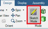
- Go to Design, Sketch Mode, and select X-Y plane.
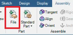
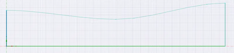
- In the Assembly tab, we have something called File to import the "Nozzle_shape_coordinates.txt" file which contains C_D nozzle shape co-ordinate points created by our MATLAB code. Close curve using line command finally sketch looks like half symmetry 2-D C_D nozzle.
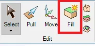
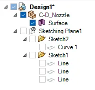
- Use the Fill tool to create a 2-D surface from the above curves.
- Add 2-D surface to the new component. Hide the sketching plane & curves, suppress them for physics.
- Meshing:
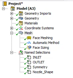
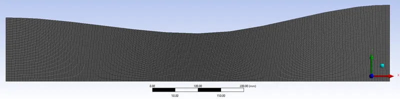
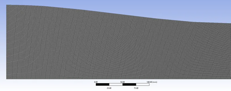
- The 2-D model created in the geometry section meshed in the mesh mode of Ansys component systems.
- Meshing is nothing but converting an infinite number of particles to model into a finite number of particles. The
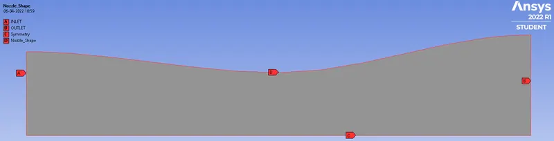
details of mesh were Physics being solved in each and every cell. physics nothing but governing equations. - Create Named sections for the edges:
- Insert Automatic, Face Meshing and Face Sizing methods.
- In the Automatic method create a Quadrilateral Dominant mesh
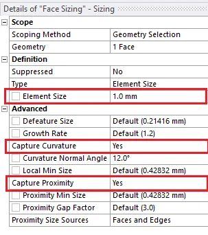
- Under the face sizing method element size is set to 2 millimeter. Proximity and Curvature option were selected since the nozzle is a curved object.
- Mesh:
- Element quality:
- Under quality, meshing smoothing was set to high.
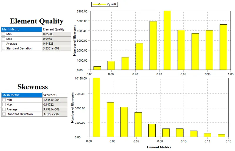
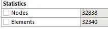
- Therefore the number of Nodes was calculated as 32,838 and the number of Elements was 32340.
- Setup:
- Using Double precision for accurate results.
-
General - Solver Type: Density-Based
- 2D Space: Planer
- Time: Steady
Physics - Energy Equation: On
- Viscous Model: Inviscid
Materials - Density: Ideal-gas
- Specific heat: `C_p = 1006.43` `(J/(kg-K))`
- Molecular Weight `M_w = 28.966` `(kg)/(k.mol)`
- `gamma` = 1.4
Cell Zone Conditions - Operating conditions
- Operating pressure = 0 Pa
-
- Calculation of Stagnation Properties:
- Based on the inlet conditions provided calculating Stagnation parameters using stagnation equations 7,8 & 9.
- Ideal Gas
- Inlet conditions
- Inlet Pressure = 200000 Pa
- Inlet Temperature = 300 K
- Inlet Velocity = 175 m/s
-
% Stagnation property calculation clear all; close all; clc %% Inlet Conditions P_i = 2000000; % Inlet Pressure Pa 2 bar T_i = 300; % Inlet Temeperatue K V = 175; % Inlet Velocity m/s %% Ideal Gas properties & Density calculation C_p = 1006.43; % Specific heat j/kg-K gamma = 1.4; % Gas index Cp/Cv R = 8.314463; %Universal gas constant J/(mol-K) Mol_mass = 0.028966; % Molecular weight Kg/mole % Density of air Kg/m^3 Rho_i = (Mol_mass*P_i)/(R*T_i); %% stagnation properties T_o = T_i + (V^2/(2*C_p)); % Stagnation Temperature P_o = P_i*((T_o/T_i)^(gamma/(gamma-1))); % Stagnation Pressure Rho_o = Rho_i*((T_o/T_i)^(1/(gamma-1))); % Stagnation Density Stagnation = fopen('Stagnation_values.txt','w'); fprintf(Stagnation,'stagnation propertiesn'); fprintf(Stagnation,'Stagnation Temperature = %f Kn',T_o); fprintf(Stagnation,'Stagnation Pressure = %f Pan',P_o); fprintf(Stagnation,'Stagnation Density = %f Kg/m^3n',Rho_o); -
output
stagnation properties
Stagnation Temperature = 315.214670     K
Stagnation Pressure    = 2378088.851114     Pa
Stagnation Density     = 26.283063     Kg/m^3
- Boundary Conditions
-
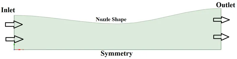
Inlet: Pressure Inlet
- Gauge Total pressure
- stagnation pressure
- 2378088.8511 Pa
- Supersonic/Initial gauge pressure
- 200000 Pa
- Total Temperature
- Stagnation temperature
- 315.214 K
- Gauge Total pressure
-
Supersonic
Shock Flow
Outlet: pressure outlet
- Gauge Pressure
- 282634.07026 Pa
- Back Flow Total Temperature
- 171.521 K
Outlet: pressure outlet
- Gauge Pressure
- 1600000 Pa
- Back Flow Total Temperature
- 171.521 K
- Gauge Pressure
-
Symmetry: Symmetry
-
Nozzle_Shape: wall
-
- Using Double precision for accurate results.
- Solution:
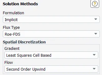
- Solution methods:
- Solution Controls:
- Courant number: 5
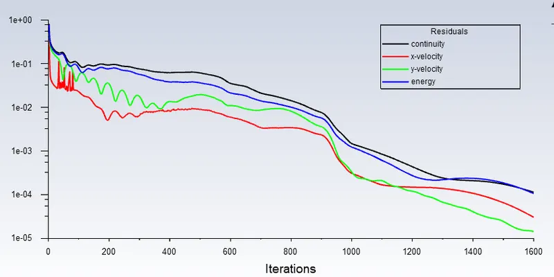
- Residuals:
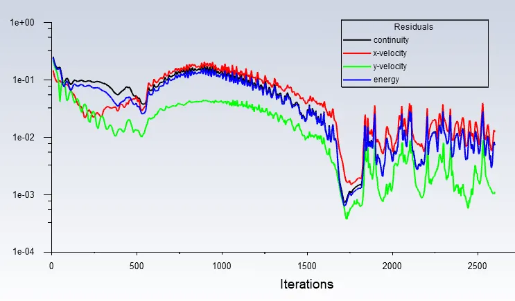
- Convergence criteria is set to 1e-6 for all variables.
- Surface Report Definition:
- Creating Area-Weighted Average reports for flow variables.
- Initialization:
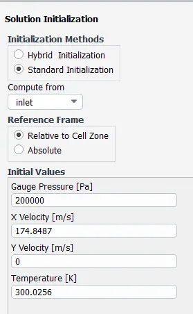
- Standard Initialization, Compute from Inlet.
- Area Weighted average reports:
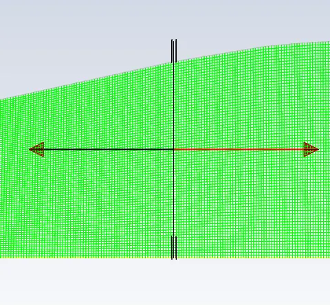
- Create 15 section lines over a length of the domain X, at each section calculate the area-weighted average of flow variables.
- Run Calculations:
- The number of iterations for the supersonic case is = 1600.
- The number of iterations for the Shockwave case is = 2600.
- Solution methods:
4.2 Results of Supersonic Case:
- Residuals:
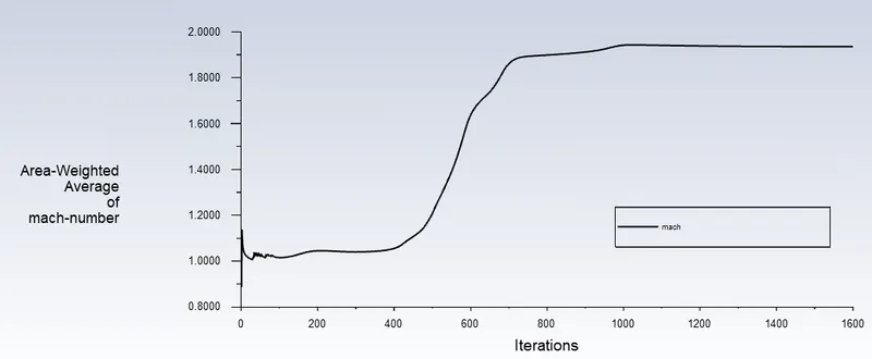
- Mach Number:
- Mach number is increasing gradually from inlet to outlet. The maximum value is at the outlet is 1.9353 and the minimum value is at the inlet is 0.5034, and at the throat it is 0.9705.
- Mach number is increasing gradually from inlet to outlet. The maximum value is at the outlet is 1.9353 and the minimum value is at the inlet is 0.5034, and at the throat it is 0.9705.
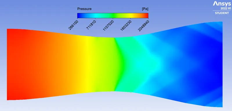
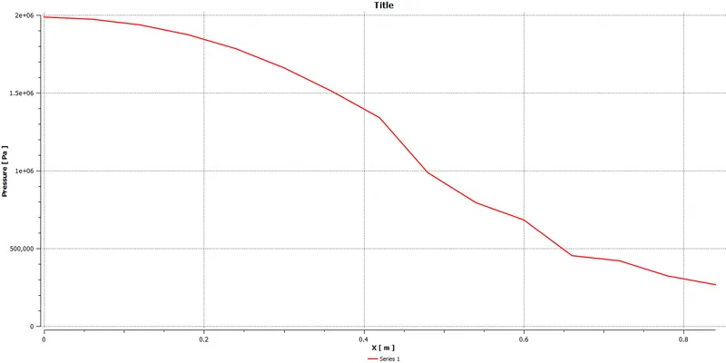
- Pressure Variation:
- Pressure goes on decreasing from Inlet to the outlet. It is maximum at the inlet section and minimum at the outlet section. The maximum pressure at the inlet is 2002030.1 Pa, the minimum pressure at the outlet is 342976.62 Pa and at the throat it is 1300787.3 Pa.
- Pressure goes on decreasing from Inlet to the outlet. It is maximum at the inlet section and minimum at the outlet section. The maximum pressure at the inlet is 2002030.1 Pa, the minimum pressure at the outlet is 342976.62 Pa and at the throat it is 1300787.3 Pa.
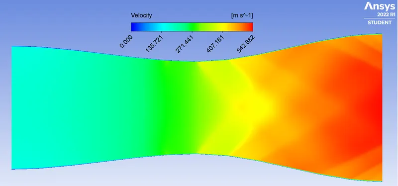
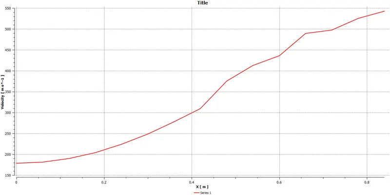
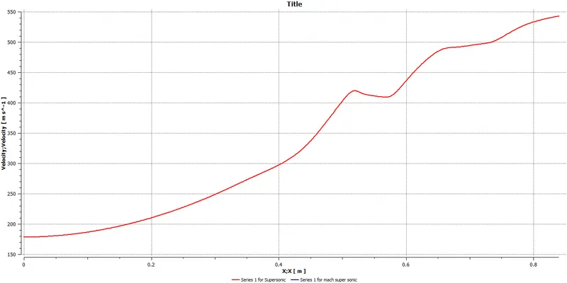
- Velocity Variation:
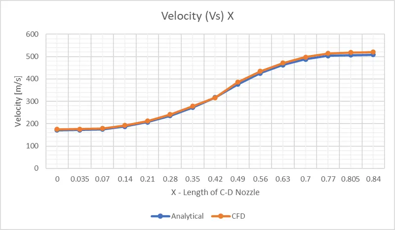
- Velocity goes on increasing from Inlet to the outlet. It is minimum at the inlet section and maximum at the outlet section. Velocity is equal to the sonic velocity at the throat. The maximum velocity at the outlet is 519.9595 m/s, the minimum velocity at the inlet is 174.3429 m/s, and at the throat it is 316.6601 m/s.
- Velocity goes on increasing from Inlet to the outlet. It is minimum at the inlet section and maximum at the outlet section. Velocity is equal to the sonic velocity at the throat. The maximum velocity at the outlet is 519.9595 m/s, the minimum velocity at the inlet is 174.3429 m/s, and at the throat it is 316.6601 m/s.
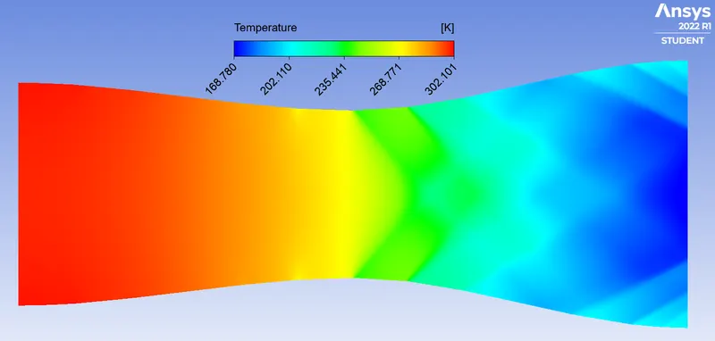
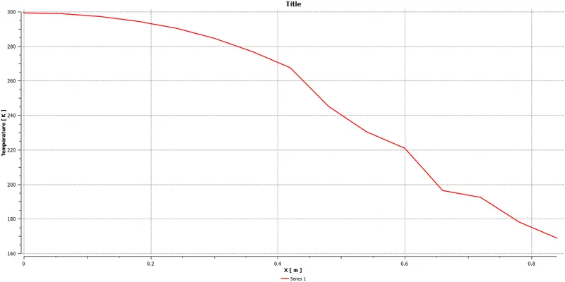
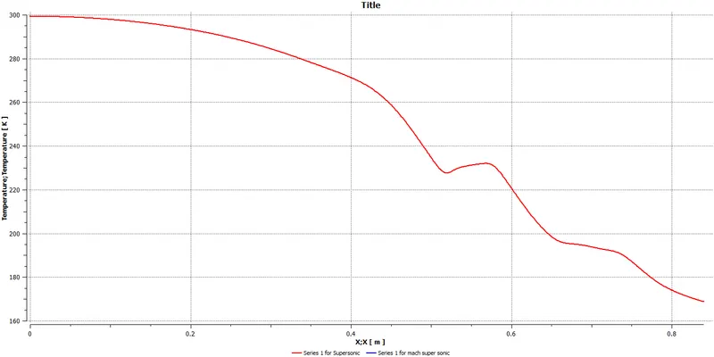
- Temperature Variation:
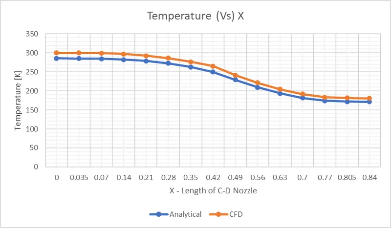
- Temperature variation is similar to pressure variation. It is maximum at the inlet and minimum at the outlet. The maximum value of temperature is 300.1055 K and the minimum value of temperature is 180.6579 K, and at the throat it is 265.3230 K.
- Temperature variation is similar to pressure variation. It is maximum at the inlet and minimum at the outlet. The maximum value of temperature is 300.1055 K and the minimum value of temperature is 180.6579 K, and at the throat it is 265.3230 K.
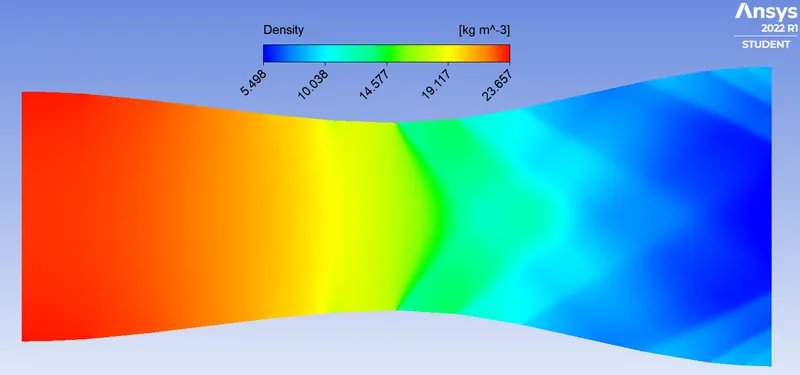
- Density Variation:
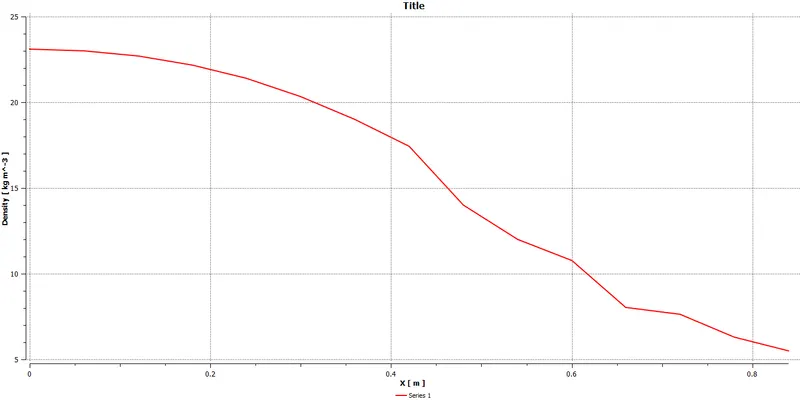
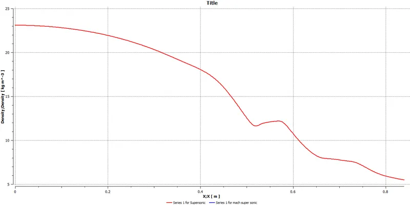
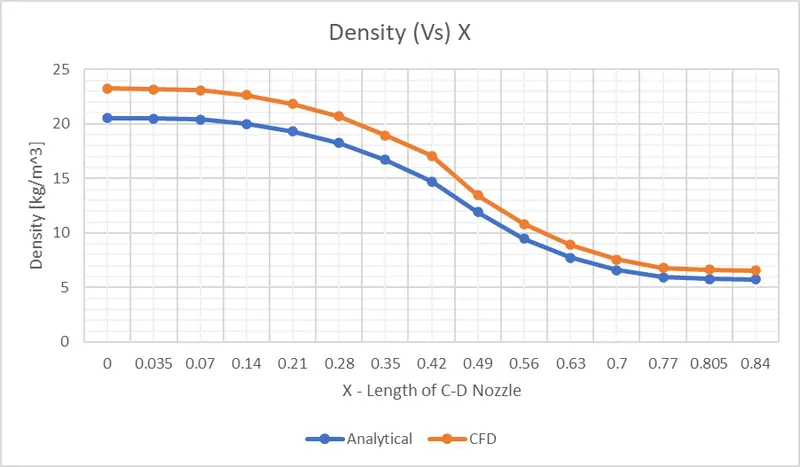
- The density of the flow is maximum at the inlet and minimum at the outlet. The maximum value of density is 23.2405 kg/m3 and the minimum value is 6.5523 kg/m3, and at the throat it is 17.0713 kg/m3.
- The density of the flow is maximum at the inlet and minimum at the outlet. The maximum value of density is 23.2405 kg/m3 and the minimum value is 6.5523 kg/m3, and at the throat it is 17.0713 kg/m3.
- Supersonic CFD simulation Results:
- Area-weighted average values at different X-sections.
-
S.No X [m] `A/A^**` Mach Number Pressure [Pa]
Temperature [K] Velocity [m/s] Density [Kg/m^3] 1 0.0000 1.3333 0.5022 2002030.1000 300.1055 174.3429 23.2405 2 0.0350 1.3267 0.5064 1996371.0000 299.8690 175.7173 23.1931 3 0.0700 1.3100 0.5153 1984214.6000 299.3476 178.6717 23.0920 4 0.1400 1.2467 0.5557 1928308.5000 296.9179 191.8935 22.6252 5 0.2100 1.1667 0.6191 1836629.1000 292.8220 212.2947 21.8510 6 0.2800 1.0867 0.7098 1699683.4000 286.4195 240.7294 20.6737 7 0.3500 1.0240 0.8356 1505410.0000 276.6501 278.4954 18.9548 8 0.4200 1.0000 0.9705 1300787.3000 265.3230 316.6601 17.0713 9 0.4900 1.0427 1.2379 933279.9400 241.4018 385.3856 13.4660 10 0.5600 1.1547 1.4594 689552.9800 221.2328 434.6591 10.8360 11 0.6300 1.3013 1.6467 524093.5100 204.5939 471.6861 8.9064 12 0.7000 1.4480 1.7940 417790.6000 191.9572 498.0559 7.5806 13 0.7700 1.5587 1.8968 358956.1700 183.5755 514.5790 6.7916 14 0.8050 1.5893 1.9227 346861.2100 181.5687 518.3679 6.6180 15 0.8400 1.6000 1.9355 342976.6200 180.6579 519.9595 6.5523
4.3 Results of Shockwave case:
- Shockwave results across the flow are as follows.
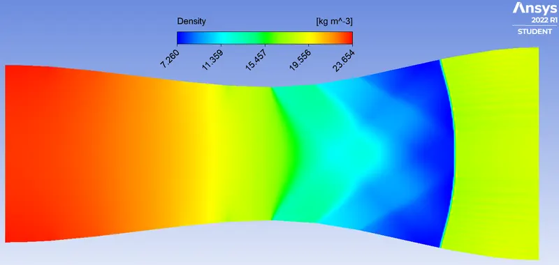
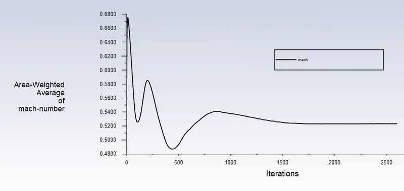
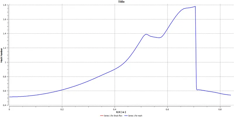
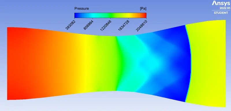
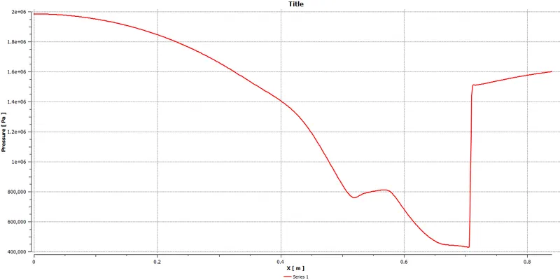
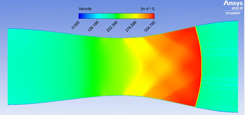
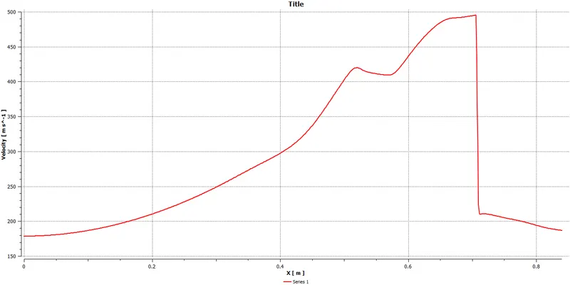
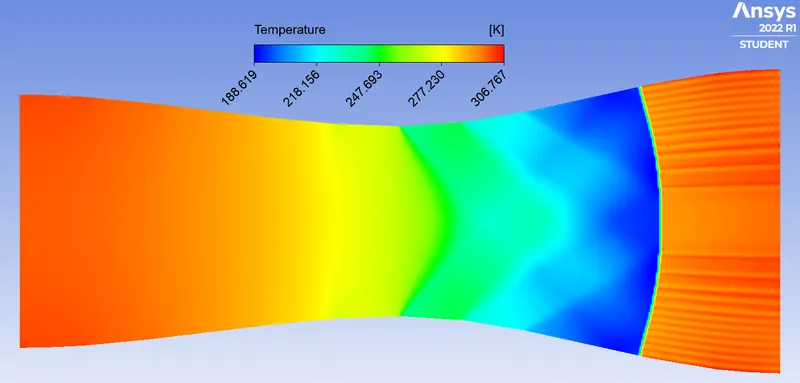
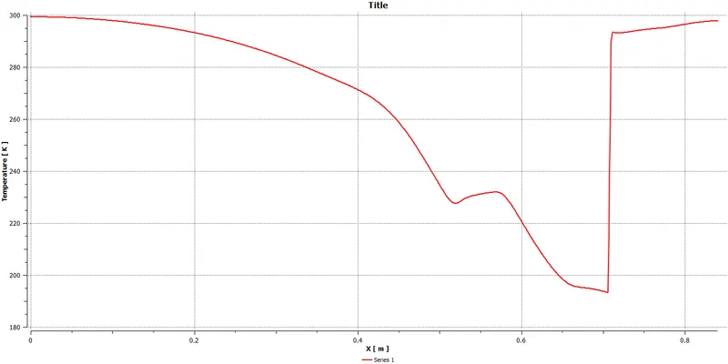
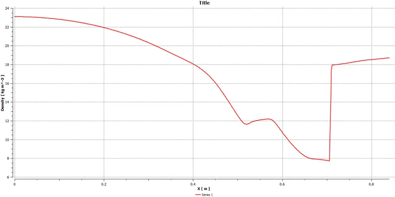
- The position of the shock is in between X = 0.7078 & 0.7088.
- Residuals:
- Mach variation due to shockwave:
- Pressure Variation due to shockwave:
- Velocity Variation due to shockwave:
- Temperature Variation due to shockwave:
- Density Variation due to shockwave
- Shockflow CFD simulation Results:
- Area-weighted average values at different inlet,Outlet, Before and After the shock.
-
Mach Number Pressure [Pa]
Temperature [K] Velocity [m/s] Density [Kg/m^3] Inlet X = 0 m 0.5025 2001614.8000 174.4359 300.0927 23.2373 Outlet X = 0.84 m 0.5231 1600000.0000 181.1897 298.8583 18.6490 Before Shockwave X1 = 0.6793 m 1.7525 445104.6000 490.9569 195.4605 7.9321 After Shockwave X2 = 0.7113 m 0.6019 1513099.0000 206.6844 293.8910 17.9381 Ratio X2/X1 0.3434 3.3994 0.4210 1.5036 2.2615
5.0 Conclusion:
- Through this study and analysis, we have found out the values of parameters of the nozzle by the Numerical method which is by using formulae and also using CFD simulation.
- In the divergent section, we can observe an infinite number of Mach waves, diverging from the surface this is due to a supersonic expansion fan around a convex corner, this flow fan is called Prandtl–Meyer expansion fan.
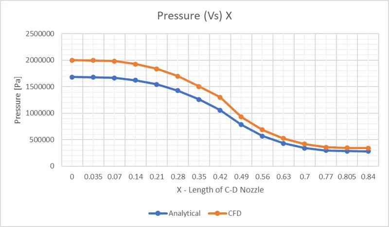
- To draw proper conclusions we have to compare both the Analytical and Simulation Results. This comparison of these values is summarized in the below tables & plots.
- Supersonic:
-
Mach Number Pressure [Pa] Temperature [K] Velocity [m/s] Density [Kg/m^2] X A_At Analytical CFD Simulation Analytical CFD Simulation Analytical CFD Simulation Analytical CFD Simulation Analytical CFD Simulation 0.000 1.3333 0.5034 0.5022 1682179.2658 2002030.1000 285.5273 300.1055 170.5284 174.3429 20.5248 23.2405 0.035 1.3267 0.5070 0.5064 1678138.4608 1996371.0000 285.3312 299.8690 171.6800 175.7173 20.4896 23.1931 0.070 1.3100 0.5162 0.5153 1667641.1817 1984214.6000 284.8201 299.3476 174.6453 178.6717 20.3979 23.0920 0.140 1.2467 0.5556 0.5557 1621707.0283 1928308.5000 282.5562 296.9179 187.2159 191.8935 19.9950 22.6252 0.210 1.1667 0.6191 0.6191 1544462.0326 1836629.1000 278.6436 292.8220 207.1506 212.2947 19.3100 21.8510 0.280 1.0867 0.7109 0.7098 1427798.7993 1699683.4000 272.4603 286.4195 235.2347 240.7294 18.2565 20.6737 0.350 1.0240 0.8390 0.8356 1261256.4623 1505410.0000 262.9745 276.6501 272.7547 278.4954 16.7088 18.9548 0.420 1.0000 1.0000 0.9705 1056553.0638 1300787.3000 249.9993 265.3230 316.9640 316.6601 14.7234 17.0713 0.490 1.0427 1.2384 1.2379 784148.6085 933279.9400 229.5836 241.4018 376.1481 385.3856 11.8990 13.4660 0.560 1.1547 1.4672 1.4594 571213.2310 689552.9800 209.7135 221.2328 425.9250 434.6591 9.4891 10.8360 0.630 1.3013 1.6604 1.6467 430070.7273 524093.5100 193.3792 204.5939 462.8527 471.6861 7.7479 8.9064 0.700 1.4480 1.8083 1.7940 343711.5427 417790.6000 181.3831 191.9572 488.1971 498.0559 6.6016 7.5806 0.770 1.5587 1.9028 1.8968 297215.2025 358956.1700 174.0049 183.5755 503.1514 514.5790 5.9506 6.7916 0.805 1.5893 1.9270 1.9227 286273.8090 346861.2100 172.1502 181.5687 506.8413 518.3679 5.7933 6.6180 0.840 1.6000 1.9353 1.9355 282634.0703 342976.6200 171.5219 180.6579 508.0850 519.9595 5.7406 6.5523 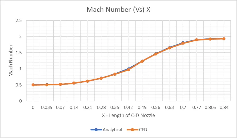
-
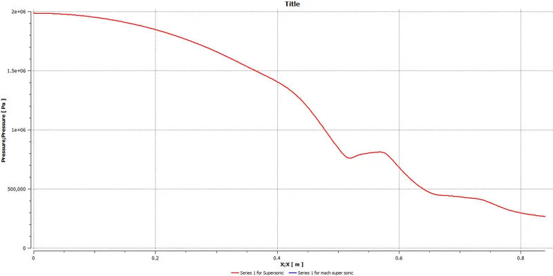
- From Mach number and Velocity plots we can observe that our analytical and CFD results are much closer and both the curves are overlapping. But, for the Pressure, Temperature & Density plots our analytical and CFD results have some deviation, this is due to Prandtl–Meyer expansion fan.
- Due Prandtl–Meyer expansion fan the flow accelerates velocity and the Mach number increases this pushed our Mach & Velocity CFD results towards analytical results. Whereas, static pressure, temperature, and density CFD results decreased further and deviated from our analytical curve.
- Since the process is isentropic, the stagnation properties (e.g. the total pressure and total temperature) remain constant across the fan.
- Shockwave:
-
Analytical solution CFD Simulation Error % Mach Number Ratio M2/M1 0.3581 0.3434 4.1050 Temperature Ratio T2/T1 1.4963 1.5036 0.4879 Pressure Ratio P2/P1 3.4161 3.3994 0.4889 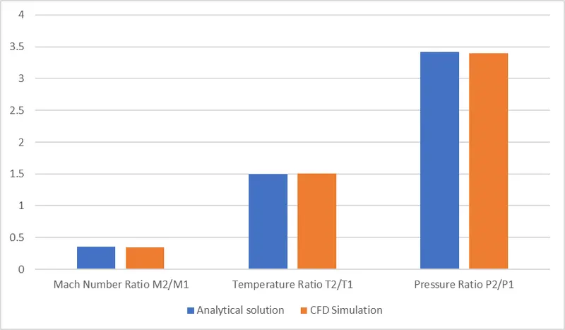
-
- From the above bar chart, we can observe that our Mach number ratio, Temperature ratio & Pressure ratio for both analytical and CFD results are similar to each other.
6.0 References:
- “Concepts and CFD Analysis of De-Laval Nozzle” by Malay S Patel, Sulochan D Mane and Manikant Raman, Dr. D.Y Patil Institute of Engineering and Technology, Pune, India.
- "CFD Analysis of De-Laval Nozzle" by Pankaj Kumar Singh, Amrendra Tripathi, Department of Aeronautical Engineering, Institute of Engineering & Technology, Bhagwant University,
Ajmer, India - "Numerical Simulation of a Convergent Divergent Supersonic Nozzle Flow" Ekanayake, E. M. Sudharshani B.Aero Eng.(Hons) (RMIT University)
- Nikhil Deshpande and Suyash Vidwans, “Theoretical and CFD Analysis of De Laval Nozzle”, vol.2, No 4, April 2014.
- Venkatesh V and C Jayapal Reddy, “Modelling and simulation of Supersonic nozzle using computational fluid dynamics,” vol. 2,2015.
- "Design and flow analysis of Convergent Divergent nozzle using CFD" S. Ramanjaneyulu, P. Sai Teja,Anil Neerukonda Institute of Technology and Sciences, Visakhapatnam, India
- "Design and Fluid Flow Analysis of Convergent-Divergent Nozzle" Yesu Ratnam.Maddu, Shaik. Saidulu, Md. Azeem3& S. Jabiulla, Department of Mechanical Engineering, ST. Peters Engineering College, Hyderabad
- CFD textbook by Jhon D. Anderson.