Finding the Global Maxima Using the Genetic Algorithm Technique

Introduction:

In real world problems, it is often needed to optimize a certain parameter, given some known physical constraints. This is where, we require an optimization algorithm, which uses the given inputs and mathematically generates a new set of population and finds the optimum function value. In this project, the Genetic Algorithm (GA) feature in MATLAB is used to find the global maxima of the Stalagmite function.

Working of a Genetic Algorithm:

Genetic Algorithm (GA) is a technique for solving optimization problems which have constraints or no constraints. It is based on the evolution theory proposed by Charles Darwin. The algorithm repetitively modifies a set of members (population) of individual solutions. At every iteration, the GA randomly selects members from the current population and uses them as parents to produce the children for the next generation. After a defined set of iterations, the population moves towards an optimum solution which is the desired result. The flow chart below illustrates the working procedure of a GA.

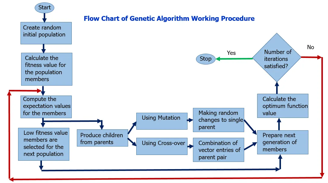
Figure 1 – Working procedure of genetic algorithm

Aim:

The aim of this project is to find the global maxima of a stalagmite function using the Genetic Algorithm feature in MATLAB. Three different methods are experimented to provide the upper and lower bounds for the GA. For each of the method, the optimum function value is plotted versus the number of iterations.

Objectives:

The main objectives of this project are to (i) understand the underlying execution procedure of the Genetic Algorithm (ii) Run the GA with no constraints on the upper and lower bounds of the search space (iii) Run the GA with constraints on the upper and lower bounds of the search space (iv) Run the GA with constraints on the upper and lower bounds of the search space along with an increased population size (vi) Adjust the population/iterations as needed to improve the accuracy of the algorithm (v) To compare the output from the different cases and discuss the results.

Governing Equations:

The main equations which are used to generate the Stalagmite function are given below.

`f(x,y)={-[f_(1,x)*f_(2,x)*f_(1,y)*f_(2,y)] }` Eqn. (1)

`f_(1,x)={sin⁡(5.1πx+0.5)}^6` Eqn. (2)

`f_(1,y)={sin⁡(5.1πy+0.5)}^6` Eqn. (3)

`f_(2,x)=exp[-4 ln⁡(2)*(x-0.0667)^2/0.64]` Eqn. (4)

`f_(2,y)=exp[-4 ln⁡(2)*(y-0.0667)^2/0.64]` Eqn. (5)

Where,

x and y are the variables that are adjusted to arrive at the random function (‘z’) value in a three-dimensional plot

f(x,y) is the random function value for the which the global maximum needs to be calculated

Main Content:

The following Matlab code finds the global maxima of the stalagmite function. The code uses the given input for the optimization search space, number of iterations, random function (stalagmite function) to arrive at the maxima of the global field. Comments are provided at each step of the code to explain the command. In this code, MATLAB’s global optimization tool box is utilized to achieve the desired results.

Program Algorithm for Main Code:

Line no.	Explanation
1	Comment line
2	Comment line
3	Comment line
4	Clear all data
5	Close all data
6	Clear command window
7	Comment line
8	define search space - 'x'
9	define search space - 'y'
10	Comment line
11	create mesh grid (x,y)
12	Comment line
13	Comment line
14	for loop-1 definition
15	for loop-2 definition
16	assigning the input vector for 'x'
17	assigning the input vector for 'y'
18	calling the stalagmite function to calculate f_stal
19	ending the second for loop
20	ending the first for loop
21	assigning figure
22	plotting the stalagmite function
23	assigning x-axis label
24	assigning y-axis label
25	assigning the plot title
26	setting the plot font size
27	removing the contour lines
28	Comment line
29	Comment line
30	assigning the number of iterations for study-1
31	starting the timer
32	Comment line
33	for loop definition for study-1
34	Comment line
35	calling the genetic algorithm to find the global maxima of the random field
36	assigning the x-value for the optimum function
37	assigning the y-value for the optimum function
38	ending the for loop
39	display the run time for study_1
40	Comment line
41	assigning figure number
42	Comment line
43	plotting the stalagmite function
44	removing the contour lines
45	hold on the plot
46	assigning x-axis label
47	assigning y-axis label
48	assigning the plot title
49	setting the plot font size
50	plotting the optimal function value (global maxima) in 3D plot
51	setting the plot font size
52	assigning x-axis label
53	assigning y-axis label
54	Comment line
55	setting the axis limits
56	Comment line
57	assigning figure number
58	plotting the optimal function value vs no. of iterations
59	assigning x-axis label
60	assigning y-axis label
61	assigning the plot title
62	setting the plot font size
63
64	Comment line
65	Comment line
66	starting the timer
67	assigning the number of iterations for study-2
68	for loop definition for study-2
69	Comment line
70	calling the genetic algorithm with upper and lower bounds to find the global maxima of the random field
71	assigning the x-value for the optimum function
72	assigning the y-value for the optimum function
73	ending the for loop
74	display the run time for study_2
75	assigning figure number
76	Comment line
77	holding on the plot
78	plotting the stalagmite function
79	removing the contour lines
80	assigning x-axis label
81	assigning y-axis label
82	assigning the plot title
83	setting the plot font size
84	plotting the optimal function value (global maxima) in 3D plot
85	assigning the plot title
86	setting the plot font size
87	assigning x-axis label
88	assigning y-axis label
89	Comment line
90	setting the axis limits
91	Comment line
92	assigning figure number
93	plotting the optimal function value vs no. of iterations
94	assigning x-axis label
95	assigning y-axis label
96	assigning the plot title
97	setting the plot font size
98
99	Comment line
100	Comment line
101	defining additional options for the GA
102	specifying the population size
103	assigning the number of iterations for study-3
104	for loop definition for study-3
105	Comment line
106	Comment line
107	calling the genetic algorithm with upper and lower bounds to find the global maxima of the random field
108	assigning the x-value for the optimum function
109	assigning the y-value for the optimum function
110	ending the for loop
111	display the run time for study_3
112	assigning figure number
113	Comment line
114	holding on the plot
115	plotting the stalagmite function
116	removing the contour lines
117	assigning x-axis label
118	assigning y-axis label
119	assigning the plot title
120	setting the plot font size
121	plotting the optimal function value (global maxima) in 3D plot
122	assigning the plot title
123	setting the plot font size
124	assigning x-axis label
125	assigning y-axis label
126	Comment line
127	setting the axis limits
128	Comment line
129	assigning figure number
130	plotting the optimal function value vs no. of iterations
131	assigning x-axis label
132	assigning y-axis label
133	assigning the plot title
134	setting the plot font size
135	Comment line

Program Algorithm for Stalagmite function:

Line no.	Explanation
1	Comment line
2	Comment line
3	function definition
4	Comment line
5	assigning 'x' variable of the input vector
6	assigning 'y' variable of the input vector
7	definition of function f1,x
8	definition of function f1,y
9	definition of function f2,x
10	definition of function f2,y
11	calculating the stalagmite function
12	ending the function
13	Comment line

Main Program Code for Genetic Algorithm Technique:

%-----------------Start of Program-----------------------
%Genetic Algorithm for  Global Optimization
%Code prepared by Srikrishna Mahadevan
%Clear and close all previous calculations, figures, etc.
clear all
close all
clc
%Defining the search space
x = linspace(0,0.6,150);
y = linspace(0,0.6,150);
%Creating a two-dimensional mesh
[xx, yy] = meshgrid(x,y);
%Evaluating the Stalagamite function
%Using Nested for loop
for i = 1:length(xx)
    for j = 1:length(yy)
        input_vector(1) = xx(i,j);
        input_vector(2) = yy(i,j);
        f_stal(i,j) = stalagmite(input_vector);
    end
end
figure(1)
surfc(xx,yy,-f_stal)
xlabel('X-value')
ylabel('Y-value')
title('Stalagmite Function');%providing plot title
set(gca,'fontsize', 20);%providing plot text size
shading interp
%GA inputs given in 3 methods
%Method-1 - Statistical Behavior
iterations_method_1 = 50;
tic
%growth,crossover,mutation
for i = 1:iterations_method_1
    %x = ga(fun,nvars)
    [inputs, fopt(i)] = ga(@stalagmite,2);%No upper or lower bounds specified
    xopt(i) = inputs(1);
    yopt(i) = inputs(2);
end
Study1_time = toc
%Plotting the results from Method-1
figure(2)
% subplot(2,1,1);%the first two digits represent the window size (2X1)
surfc(xx,yy,-f_stal)%Need to use -f_stal for the global_maxima value
shading interp
hold on
xlabel('X-value')
ylabel('Y-value')
title('Unbounded Inputs');%providing plot title
set(gca,'fontsize', 20);%providing plot text size
plot3(xopt,yopt,-fopt,'marker','o','markersize',10,'markerfacecolor','r');
set(gca,'fontsize', 20);%providing plot text size
xlabel('X-value')
ylabel('Y-value')
%setting the axis limits
axis([0 0.6 0 0.6])
% subplot(2,1,2)
figure(3)
plot(-fopt,'black','linewidth',3)
xlabel('Iterations')
ylabel('Function minimum')
title('Optimal Function Value')
set(gca,'fontsize', 20);%providing plot text size

%Method-2
%Statistical behavior with upper and lower bounds
tic
iterations_method_2 = 50;
for i = 1:iterations_method_2
    %x = ga(fun,nvars,A,b,Aeq,beq,lb,ub)
    [inputs, fopt(i)] = ga(@stalagmite,2,[],[],[],[],[0;0],[0.3;0.3]);%[] - equality or inequality constraints
    xopt(i) = inputs(1);
    yopt(i) = inputs(2);
end
Study2_time = toc
figure(4)
% subplot(2,1,1)
hold on
surfc(xx,yy,-f_stal)
shading interp
xlabel('X-value')
ylabel('Y-value')
title('Statistical Behavior - Bounded Inputs');%providing plot title
set(gca,'fontsize', 20);%providing plot text size
plot3(xopt,yopt,-fopt,'marker','o','markersize',5,'markerfacecolor','r');
title('Bounded Inputs')
set(gca,'fontsize', 20);%providing plot text size
xlabel('X-value')
ylabel('Y-value')
%setting the axis limits
axis([0 0.6 0 0.6])
% subplot(2,1,2)
figure(5)
plot(-fopt,'b','linewidth',3)
xlabel('Iterations')
ylabel('Function minimum')
title('Optimal Function Value')
set(gca,'fontsize', 20);%providing plot text size

%Method-3
%Increasing the GA iterations
options = optimoptions('ga');
options = optimoptions(options,'PopulationSize',170);
iterations_method_3 = 50;
tic
for i = 1:iterations_method_3
%x = ga(fun,nvars,A,b,Aeq,beq,lb,ub,nonlcon,options)
    [inputs, fopt(i)] = ga(@stalagmite,2,[],[],[],[],[0;0],[0.3;0.3],[],[],options);%[] - equality or inequality constraints
    xopt(i) = inputs(1);
    yopt(i) = inputs(2);
end
Study3_time = toc
figure(6)
% subplot(2,1,1)
hold on
surfc(xx,yy,-f_stal)
shading interp
xlabel('X-value')
ylabel('Y-value')
title('Bounded Inputs with Increased Population');%providing plot title
set(gca,'fontsize', 20);%providing plot text size
plot3(xopt,yopt,-fopt,'marker','o','markersize',5,'markerfacecolor','r');
title('Bounded Inputs')
set(gca,'fontsize', 20);%providing plot text size
xlabel('X-value')
ylabel('Y-value')
%setting the axis limits
axis([0 0.6 0 0.6])
% subplot(2,1,2)
figure(7)
plot(-fopt,'r','linewidth',3)
xlabel('Iterations')
ylabel('Function minimum')
title('Optimal Function Value')
set(gca,'fontsize', 20);%providing plot text size
%-----------------End of Program-----------------------

Genetic Algorithm (GA) Syntax:

The syntax for the GA is given below.

[inputs, fopt(i)] = ga(@stalagmite,2,[],[],[],[],[0;0],[0.3;0.3],[],[],options)

On the left hand side, the inputs (i.e. x and y values) are provided first followed by the optimal function value that is predicted by the GA. On the right hand side, we have the calling of the stalagmite function (i.e. field with random peaks) to ascertain the global maxima of the random field. Next to the function calling, the number of inputs (i.e. 2 in this case) are provided. The next four empty brackets are for including any equality/inequality constraints. After this, the lower and upper bounds are specified (i.e. 0;0.3 in this case). In addition, one can specify the population size using the options field.

Program Code for Stalagmite Function:

%---------------------------------Start of Function--------------------------
%Function to generate a random field with multiple peaks
function [f] = stalagmite(input_vector)
%Defining the search space
x=input_vector(1);
y=input_vector(2);
f1_x = sin((5.1*pi().*x)+0.5).^6;
f1_y = sin((5.1*pi().*y)+0.5).^6;
f2_x = exp(-4*log(2)*(((x-0.0667).^2)/0.64));
f2_y = exp(-4*log(2)*(((y-0.0667).^2)/0.64));
f = -(f1_x.*f2_x.*f1_y.*f2_y);%f(x,y) is the 'z' value
end
%---------------------------------End of Function--------------------------

Results and Discussion:

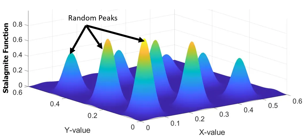
Figure 2 - Stalagmite Function

The stalagmite function generated using Equations 1-5 is shown in Fig. 2. As the name implies, stalagmite peaks point upward from the datum surface and hence the negative sign in the function definition. Since the Genetic Algorithm can only find the global minima, we have to flip the absolute value of the peak as predicted by the GA. This is done in the main code.

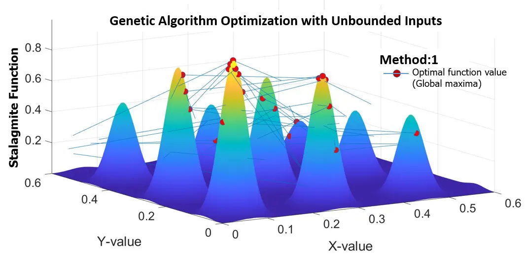
Figure 3 - GA optimization with unbounded inputs [Method-1]

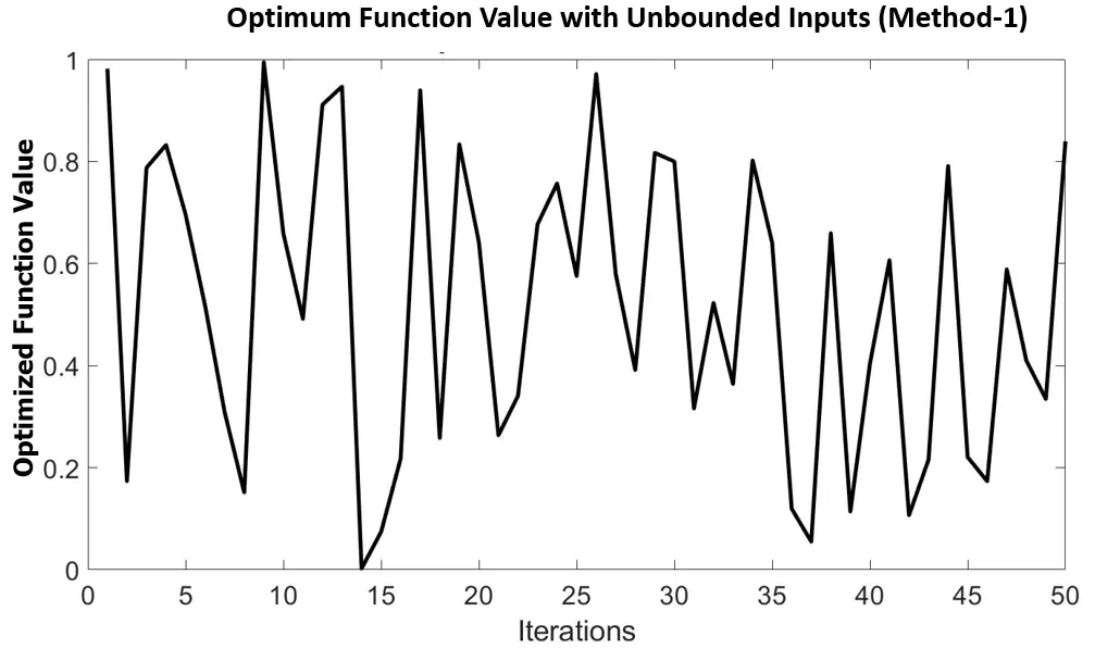
Figure 4 - Predicted optimal function values for Method-1

As mentioned earlier in this project report, three different studies (methods) were used to provide the required inputs for the genetic algorithm. In the first study shown in Figure 3 and 4, no bounds were imposed on the search space and so the algorithm will look for the optimum function value in the entire search space. Figure 3 shows the predicted maxima values using red markers superimposed on the stalagmite function. It is evident that the prediction accuracy is poor since the markers are highly scattered. In Fig. 4, the optimum function value (or the global maxima value) is plotted versus the number of iterations. One can clearly see the drastic variation (between 0 and 1) in the predicted maxima values. This result is not useful as the solution does not converge to a single optimum value. The time taken for running the program is given in table-1.

Table 1 - Run time for various Studies:

Method/Study	Time taken to run [sec.]
1	12.51
2	15.43
3	45.49

As seen in Table-1, the run times are close between study-1 and study-2 while study-3 has taken 3 times that of study-2 to complete. This is because of the increased population size which in turn increases the number of members at every iteration. On one hand, while the solution accuracy is increased when using a higher population size, the run times can be much higher. So, one needs to carefully evaluate the problem before choosing the appropriate number of iterations and population size.

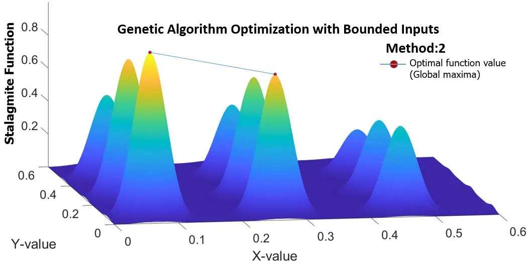
Figure 5 - GA optimization with unbounded inputs [Method-2]

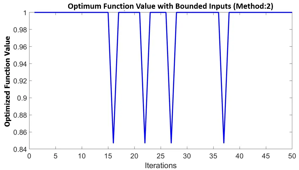
Figure 6 - Predicted optimal function values for Method-2

In study-2, both lower and upper bounds (0 to 0.3) were added to the genetic algorithm (GA) syntax so that there is control over the algorithm search space. By doing this, it was observed that the results got much better as seen in Fig. 4. The global maxima peaks have now narrowed down to two values as seen in Fig. 4. This is indicative of the clarity that the bounded inputs provide the GA. Moving on to Fig. 5, it can be noted that the optimum function value lies very close to 0.85. These results can be improved by stepping up the initial population size as this will increase the accuracy of the prediction.

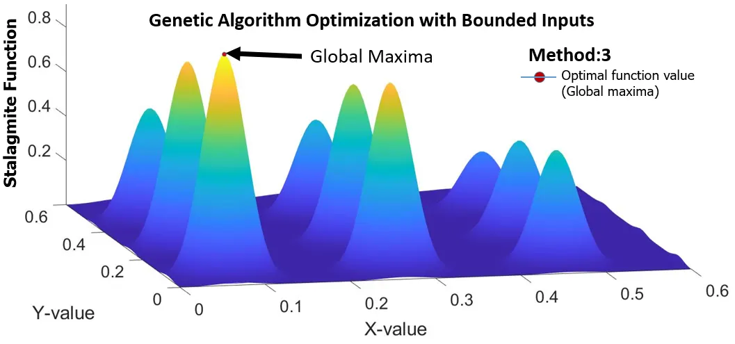
Figure 7 - GA optimization with unbounded inputs [Method-3]

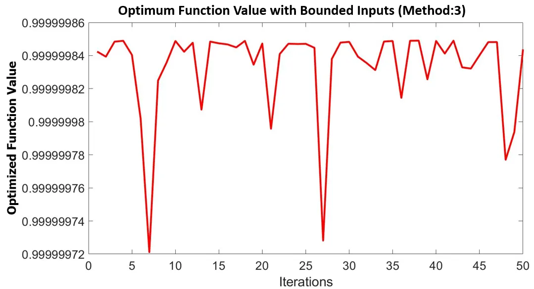
Figure 8 - Predicted optimal function values for Method-3

In the final study (method-3), in addition to the lower and upper bounds used in study-2, a population size of 170 is used. This is higher than the default population size used in the GA. Looking at the results in Fig. 6, it is interesting to note that the global maxima (single peak) has been well predicted by the GA. This reinforces the essentiality of a higher population size during the GA execution. In Fig. 6, the optimal function value is shown versus the number of iterations. It is understood that the various peaks have negligible difference in their amplitudes (i.e. change is in the seventh decimal place).

Conclusions:

In this project, the genetic algorithm (GA) technique in Matlab was used to find the global maxima of a random field with various peak values. Similary, as a future work, one can experiment the GA technique with different types of problems where a certian optimum value is required within a certain search space. It was observed that the lower and upper bounds significantly enhance the accuracy and convergence of the solution.

References:

1. Genetic Algorithm working procedure, Matlab Documentation, The MathWorks Inc., 2020