Mathematical Formulation of Curve Fit

Introduction:

This project is about fitting a mathematical function which closely approximates the raw data set (i.e. actual data). The mathematical function uses the ‘X’ values of the data set to predict the values of the raw data. A curve (linear or polynomial) is used to fit the raw data as best as possible so that the data can be expressed as a mathematical function. In some circumstances, the curve fit is also used to extrapolate the data where measurements are not available.

Aim:

The aim of this project is to perform a curve fit to a data set which provides Specific heat at constant pressure (C_p) versus Temperature. MATLAB’s curve fitting toolbox is used to arrive at the best curve fit after careful evaluation of the data trend.

Governing Equations:

The main equations which are associated with the curve fitting and error quantification process are given below.

`Y=f(X)=aX^n+bX^(n-1)+cX^(n-2)+⋯+C` Eqn. [1]

Where,

a,b,c - polynomial coefficients

C – polynomial constant

Y – polynomial function

n – exponent (obtained from the curve fit)of the independent variable

In order to quantify the goodness of fit, we use the ‘R-square’ value, which is essentially the square of the correlation between the actual data and the predicted data. It is calculated as follows.

Error in the curve fit (E) = `Y(i)-f(X(i))` Eqn. [2]

Sum of the squares of the error (SSE) = `[Y(i)-f(X(i))]^2` Eqn. [3]

Sum of the squares of the regression (SSR) = `[f(X(i))-barY]^2` Eqn. [4]

Total sum of the squares (SST) = SSE + SSR Eqn. [5]

R-square (R²) = SSR/SST Eqn. [6]

Where,

`barY` – arithmetic mean of the actual data set

The value of R² is between 0 and 1. A perfect match curve fit is given by R² = 1 and poor match curve fit is given by R² = 0.

Objectives:

The main objectives of this project are to (i) understand the mathematical background in using a curve fit (ii) Curve fit a raw data set using a linear fit (iii) Curve fit a raw data set using a cubic fit (iv) Curve fit a raw data set using a split-wise fit, using a combination of linear and quadratic fits (v) Quantify the goodness of fit and why one fit is better than the other (vi) Differentiate between best and perfect curve fits.

Main Content:

The following Matlab code is written to Comments are provided at each step of the code to explain the command. The code uses the given raw data for Cp vs temperature and fits a linear, cubic and split-wise curve fit using MATLAB’s curve fitting tool box. In addition, the code calculates the goodness of the curve fit using the least squares method.

Program Algorithm for Main Code:

Line No.	Explanation
1-4	Code title and description
5-7	Clear all previous data/screen and close windows of previous code execution
8-10	loading raw data for Cp and temperature
11-13	assigning the columns to the variables appropriately
17,18	calculating the curve fit coefficients for the linear fit
19,20	Predicted Cp values using the Linear fit
21-23	calculating the curve fit coefficients for the cubic fit
24,25	Predicted Cp values using the Cubic fit
29,30	Start and end index of data set-A of the split-wise curve fit
31,32	assigning the Cp and Temperature column data
34,35	Start and end index of data set-B of the split-wise curve fit
36,37	assigning the Cp and Temperature column data
39,40	Start and end index of data set-C of the split-wise curve fit
41,42	assigning the Cp and Temperature column data
46,47	Calculating the curve fit coefficients and predicted Cp for Data set - A
50,51	Calculating the curve fit coefficients and predicted Cp for Data set - B
54,55	Calculating the curve fit coefficients and predicted Cp for Data set - C
57	setting the figure count
58	plotting the raw data
59	providing plot title
60	providing plot text size
62	plotting the linear fit data
63	plotting the cubic fit data
64	providing plot legend
65-67	Providing labels for the X and Y axis
68-69	Setting axis limits
70-72	Turning the major and minor grid lines ON in the plot
76	setting the figure count
77	plotting the raw data
78	providing plot title
79	providing plot text size
81	plotting the linear fit-A of split-wise curve fit
82	plotting the quadratic fit-A of split-wise curve fit
83	plotting the linear fit-C of split-wise curve fit
84	providing plot legend
85-87	Providing labels for the X and Y axis
88-89	Setting axis limits
90-92	Turning the major and minor grid lines ON in the plot
96-108	Using For loop for calculating the accuracy of the curve fit for entire data set-linear and cubic Using Least squares method SSE – Calculating the sum of the squares of the error SSR – Calculating the sum of the squares of the regression SST - Calculating the total sum of the squares of the curve fit
112-114	Calculating the sum of SSE, SSR, SST
115	Calculating R square value for the cubic fit
117-119	Calculating the sum of SSE, SSR, SST
120	Calculating R square value for the linear fit
125-132	Using For loop-1 for calculating the accuracy of the curve fit for the split-wise curve fit (linear-A) Using Least squares method
134-137	Calculating R square value for the linear-A fit
141-148	Using For loop-2 for calculating the accuracy of the curve fit for the split-wise curve fit (Quadratic-B) Using Least squares method
151-154	Calculating R square value for the Quadratic-B fit
158-165	Using For loop-3 for calculating the accuracy of the curve fit for the split-wise curve fit (linear-C) Using Least squares method
168-171	Calculating R square value for the linear-C fit
175-179	Provide value for the polynomial degree for all curve fits
181	setting the figure count
183	plotting the R-square value for the cubic fit
184	providing plot title
185	providing plot text size
188	plotting the R square value for linear of split-wise curve fit
191	plotting the R square value for linear fit-A of split-wise curve fit
192	plotting the R square value for quadratic fit-A of split-wise curve fit
193	plotting the R square value for linear fit-C of split-wise curve fit
194-196	providing plot legend
198-199	Providing labels for the X and Y axis
200-202	Setting axis limits
204-205	Turning the major and minor grid lines ON in the plot

Main Code:

%-----------------Start of Program-----------------------
%Curve fitting in Matlab
%Code prepared by Srikrishna Mahadevan
%Clear and close all previous calculations, figures, etc.
clear all
close all
clc
%Inputs for the Cp vs Temperature variation
%loading raw data for Cp and temperature
Cp_data = load('Cp_vs_temp_data');
%assigning the columns to the variables appropriately
temperature = Cp_data(:,1);
Cp = Cp_data(:,2);
%Curve fit details
%Cp = (a*T^2)+(b*T)+c
%Linear fit for the entire data
%calculating the curve fit coefficients
coeffs_L = polyfit(temperature,Cp,1);
%Predicted Cp values using the Linear fit
Curve_fit_Cp_L = polyval(coeffs_L, temperature);
%Cubic fit for the entire data
%calculating the curve fit coefficients
coeffs_P3 = polyfit(temperature,Cp,3);
%Predicted Cp values using the Cubic fit
Curve_fit_Cp_P3 = polyval(coeffs_P3, temperature);
%Splitting the data set into multiple parts for 
%better curve fit
%Data set - A 
A1 = 1;%start index 
A2 = 465;%end index 
Cp_A = Cp(A1:A2);%assigning the Cp column data
Temp_A = temperature(A1:A2);%assigning the temp. column data
%Data set - B 
B1 = 465;%start index 
B2 = 1051;%end index
Cp_B = Cp(B1:B2);%assigning the Cp column data
Temp_B = temperature(B1:B2);%assigning the temp. column data
%Data set - C 
C1 = 1051;%start index 
C2 = 3200;%end index
Cp_C = Cp(C1:C2);%assigning the Cp column data
Temp_C = temperature(C1:C2);%assigning the temp. column data

%Calculating the curve fit coefficients and predicted Cp 
%for Data set - A 
coeffs_A = polyfit(Temp_A,Cp_A,1);
Curve_fit_Cp_A = polyval(coeffs_A, Temp_A);
%Calculating the polynomial coefficients and predicted Cp 
%for Data set - B
coeffs_B = polyfit(Temp_B,Cp_B,2);
Curve_fit_Cp_B = polyval(coeffs_B, Temp_B);
%Calculating the polynomial coefficients and predicted Cp 
%for Data set - C
coeffs_C = polyfit(Temp_C,Cp_C,1);
Curve_fit_Cp_C = polyval(coeffs_C, Temp_C);
%Comparing the Linear and Cubic fit data with the actual data
figure(1)
plot(temperature,Cp,'o','color','blue','linewidth',1);%plotting the raw data
title('Specific Heat at Constant Pressure vs Temperature');%providing plot title
set(gca,'fontsize', 20);%providing plot text size
hold on
plot(temperature,Curve_fit_Cp_L,'red','linewidth',4);%plotting the linear fit data
plot(temperature,Curve_fit_Cp_P3,'black','linewidth',4);%plotting the cubic fit data
legend('Raw Data','Linear fit','Cubic fit');%providing the legend
%providing labels for the x and y axis
xlabel('Temperature [K]')
ylabel('Specific Heat at Constant Pressure [J/kgK]')
%setting the axis limits
% axis([0 4 0.5 2])
%enabling the grid display
grid on
grid minor

%Comparing the curve fit data with the actual data for 
%Splitwise curve fit
figure(2)
plot(temperature,Cp,'o','color','blue','linewidth',1);%plotting the raw data
title('Specific Heat at Constant Pressure vs Temperature');%providing plot title
set(gca,'fontsize', 20);%providing plot text size
hold on
plot(Temp_A,Curve_fit_Cp_A,'red','linewidth',4);%plotting splitwise fit for data set-A
plot(Temp_B,Curve_fit_Cp_B,'green','linewidth',4);%plotting splitwise fit for data set-B
plot(Temp_C,Curve_fit_Cp_C,'black','linewidth',4);%plotting splitwise fit for data set-C
legend('Raw Data','Linear fit-1','Quadratic fit','Linear fit-2');%providing the legend
%providing labels for the x and y axis
xlabel('Temperature [K]')
ylabel('Specific Heat at Constant Pressure [J/kgK]')
%setting the axis limits
% axis([0 4 0.5 2])
%enabling the grid display
grid on
grid minor

%Using For loop for calculating the accuracy of the curve fit 
%for entire data set-linear and cubic 
%Using Least squares method
for i=1:3200%initialising the index range
    %for entire data set-linear
    %Calculating the sum of the squares of the error
    SSE_L(i) = (Cp(i) - Curve_fit_Cp_L(i)).^2;%linear fit
    SSE_P3(i) = (Cp(i) - Curve_fit_Cp_P3(i)).^2;%cubic fit
    %Calculating the sum of the squares of the regression
    SSR_L(i) = (Curve_fit_Cp_L(i) - mean(Cp)).^2;%linear fit
    SSR_P3(i) = (Curve_fit_Cp_P3(i) - mean(Cp)).^2;%cubic fit
    %Calculating the total sum of the squares of the curve fit
    SST_L(i) = (SSR_L(i) + SSE_L(i));%linear fit
    SST_P3(i) = (SSR_P3(i) + SSE_P3(i));%cubic fit
end
%Calculating R square value for the Cubic fit
%R square is the square of the correlation between 
%the actual values and the predicted data
SSE_P3_sum = sum(SSE_P3);%calculating sum of SSE
SSR_P3_sum = sum(SSR_P3);%calculating sum of SSR
SST_P3_sum = SSR_P3_sum + SSE_P3_sum;%calculating sum of SST
R_sq_P3 = (SSR_P3_sum/SST_P3_sum);%calculating R square value
%Calculating R square value for the linear fit
SSE_L_sum = sum(SSE_L);%calculating sum of SSE
SSR_L_sum = sum(SSR_L);%calculating sum of SSR
SST_L_sum = SSR_L_sum + SSE_L_sum;%calculating sum of SST
R_sq_L = (SSR_L_sum/SST_L_sum);%calculating R square value

%Using For loop for calculating the accuracy of the curve fit 
%the splitwise curve fit - Data set-A - Linear fit
%Using Least squares method
for i=1:465%initialising the index range
    %Calculating the sum of the squares of the error
    SSE_A(i) = (Cp_A(i) - Curve_fit_Cp_A(i)).^2;
    %Calculating the sum of the squares of the regression
    SSR_A(i) = (Curve_fit_Cp_A(i) - mean(Cp_A)).^2;
    %Calculating the total sum of the squares of the curve fit
    SST_A(i) = (SSR_A(i) + SSE_A(i));
end
%Calculating R square value for the Linear fit-A
SSE_A_sum = sum(SSE_A);%calculating sum of SSE
SSR_A_sum = sum(SSR_A);%calculating sum of SSR
SST_A_sum = SSR_A_sum + SSE_A_sum;%calculating sum of SST
R_sq_A = (SSR_A_sum/SST_A_sum);%Calculating R square value
%Using For loop for calculating the accuracy of the curve fit 
%the splitwise curve fit - Data set-B - Quadratic fit
%Using Least squares method
for j=465:1051%initialising the index range
    %Calculating the sum of the squares of the error
    SSE_B(i) = (Cp_B(i) - Curve_fit_Cp_B(i)).^2;
    %Calculating the sum of the squares of the regression
    SSR_B(i) = (Curve_fit_Cp_B(i) - mean(Cp_B)).^2;
    %Calculating the total sum of the squares of the curve fit
    SST_B(i) = (SSR_B(i) + SSE_B(i));
end
%Calculating R square value for the quadratic curve fit
%for data set-B
SSE_B_sum = sum(SSE_B);%calculating sum of SSE
SSR_B_sum = sum(SSR_B);%calculating sum of SSR
SST_B_sum = SSR_B_sum + SSE_B_sum;%calculating sum of SST
R_sq_B = (SSR_B_sum/SST_B_sum);%Calculating R square value
%Using For loop for calculating the accuracy of the curve fit 
%the splitwise curve fit - Data set-C - Linear fit
%Using Least squares method
for k=1051:3200%initialising the index range
    %Calculating the sum of the squares of the error
    SSE_C(i) = (Cp_C(i) - Curve_fit_Cp_C(i)).^2;
    %Calculating the sum of the squares of the regression
    SSR_C(i) = (Curve_fit_Cp_C(i) - mean(Cp_C)).^2;
    %Calculating the total sum of the squares of the curve fit
    SST_C(i) = (SSR_C(i) + SSE_C(i));
end
%Calculating R square value for the linear curve fit-2
%for data set-C
SSE_C_sum = sum(SSE_C);%calculating sum of SSE
SSR_C_sum = sum(SSR_C);%calculating sum of SSR
SST_C_sum = SSR_C_sum + SSE_C_sum;%calculating sum of SST
R_sq_C = (SSR_C_sum/SST_C_sum);%Calculating R square value

%Provide value for the polynomial degree for 
%all curve fits
deg_P3 = 3;%Fully Cubic fit
deg_L = 1;%Fully Linear fit
deg_A = 1;%Linear fit-1, part of splitwise curve fit
deg_B = 2;%Quadratic fit, part of splitwise curve fit
deg_C = 1;%Linear fit-2, part of splitwise curve fit
%Comparing the R-square values between different curve fits
figure(3)
%plotting the R-square value for the cubic fit
plot(deg_P3,R_sq_P3,'o','color','blue','linewidth',4);
title('Goodness of Curve Fit');%providing plot title
set(gca,'fontsize', 20);%providing plot text size
hold on
%plotting the R-square value for the linear fit
plot(deg_L,R_sq_L,'o','color','red','linewidth',4);
%plotting the R-square values for the splitwise fit
%Linear-A, Quadratic-B, Linear-C
plot(deg_A,R_sq_A,'o','color','black','linewidth',4);
plot(deg_B,R_sq_B,'o','color','magenta','linewidth',4);
plot(deg_C,R_sq_C,'o','color','green','linewidth',4);
%providing plot legends
legend('Cubic','Linear','Linear-1','Quadratic','Linear-2');
% legend('Cubic','Linear-A','Quadratic-B','Linear-C');
%providing labels for the x and y axis
xlabel('Degree of Curve fit [-]')
ylabel('R square value [-]')
%setting the axis limits
% axis([0 4 0.99 1])
axis([0 4 0.92 1])
%enabling the grid display
grid on
grid minor
% -----------------------End of program------------------------------

Results and Discussion:

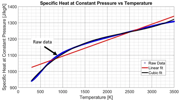
Figure 1 – Raw data fitted with linear and cubic curves

The raw data of Specific heat versus Temperature is shown using blue symbols in Fig. 1. It is evident that the trend in the raw data is non-linear. However, a linear fit is initially used to curve fit the data followed by a cubic fit (i.e. polynomial of 3^rd degree). The linear curve fit deviates significantly from the raw data, especially near the initial part of the curve. On the other hand, the cubic curve approximates the raw data reasonably well but the polynomial (mathematical function) was badly conditioned as inferred from MATLAB. Due to this issue, a split-wise method is used to approximate the raw data as shown in Fig. 2.

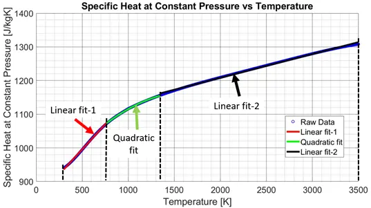
Figure 2 – Split-wise curve fit for the Raw data

As seen in Fig. 2, three different curve fits are used to predict the trend in the actual data. The main reason for this approach was because of the non-linearity in the raw data. Some parts of the raw data set are close to linear while the other part is non-linear. The initial part of the curve is approximated using linear fit (indicated in red) for index range - 1 to 465. There is a good match between the actual data and the predicted values. For the second part of the data set, a quadratic fit is used (indicated in green) for index range - 465 to 1051. The match is excellent between the actual data and the predicted values. A linear fit is used to estimate the last portion of the data set (indicated in black) for index range - 1051 to 3200. The accuracy of the curve fit appears to be very good.

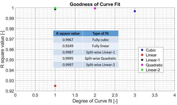
Figure 3 – Quantification of curve fit accuracy

The accuracy of the curve fit is quantified using the R-square value as shown in Fig. 3. It is evident from Fig. 3 that the full linear fit has a lower accuracy in predicting the raw data due to the significant non-linearity in the actual data set. Alternatively, the cubic fit has a very good match with the actual data. But it was observed (during program execution) that the polynomial was badly conditioned (i.e. any small change in the data set can significantly change the coefficients of the polynomial and hence the trend). The cubic fit can be improved by splitting the data into multiple data sets and using a lower order polynomial.

So, it was necessary to try a split-wise curve fit after carefully studying the trend of the raw data. As seen from Fig. 3, the curve fit accuracy is close to 1 for the curves obtained using the split-wise method. This reiterates the essentiality of splitting any real time data set that is highly non-linear into multiple portions to obtain a reliable curve fit.

A perfect curve fit is obtained only when the curve matches the raw data exactly. It is often difficult to get this. On the other hand, a best fit curve is possible by using the split-wise method.

Conclusions:

In this project, the underlying mathematical background of curve fit was studied in detail. Multiple curve fits were tried for the given raw data set and the R-square value was calculated in each case to quantify the accuracy of the fit. The fully linear fit was not very accurate. While the cubic fit was fairly accurate, the polynomial was badly conditioned. So, the split-wise curve fit was used for the data set for which the accuracy was excellent. Therefore, it can be said that in reality, it may not be possible to obtain a perfect curve fit for all cases due to the non-linearity in the data sets. But it is possible to best estimate the raw data quantitatively using the split-wise method. Similarly, any real data can be mathematically approximated using a curve fit. As a future effort, it would be interesting to look into logarithmic curve fits.

References:

[1]. Curve fitting mathematics - https://projects.skill-lync.com/projects/Curve-Fitting-and-criterion-to-choose-best-fit-41860

[2]. Cp vs Temperature data set provided by Skill Lync