Application of Simulink and Simscape to real world problems
INTRODUCTION:
In this project, three different problems are addressed from a mathematical and physical perspective. These problems are related to day-to-day applications. Simulink/Simscape models are built to address the problem requirement. The emphasis is on the underlying mathematical and physical principles and extend this knowledge to select the Simulink/Simscape blocks judiciously.
AIM:
The aim of this project is to use the Simulink and Simscape blocks to solve three different problems involving mathematical and physical equations. In addition, it is required to understand the correct logic behind block selection in Simulink and Simscape.
OBJECTIVES:
The main objectives of this project include (i) to calculate the work done by a cutting tool on a shaping machine (ii) to create a Simulink model to calculate a mathematical function using array inputs (iii) to understand the working of a spring-mass damper system and derive the governing equation from the
Simulink model; record the transient response of the system for different values of initial displacement, body mass, damping coefficient and spring stiffness to observe the variation.
SIMULINK MODEL DESCRIPTION AND GOVERNING EQUATIONS:
(a) Work done by Cutting tool in a shaping machine:
The Simulink model for the work done by a cutting is shown in Figure-1. The inputs for the force and displacement are provided using the constant block with the variable arrays assigned from the base workspace. Since the work done by the cutting tool is the product of force and displacement (provided in (Eqn. [1]), a product block is used for array multiplication. Since the force and displacement are arrays, a summation block is required to calculate the total work done (provided in Eqn. [2]).
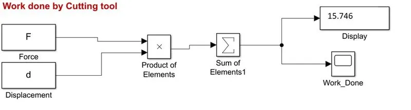
Figure 1 – Simulink model to calculate Work done by Cutting tool
Based on the available inputs for cutting tool force and displacement, the work done by the cutting tool is calculated as follows,
Work done = Force * displacement ...............Eqn. [1]
Total work done (W) = `∑_(i=1)^N(F_i d_i)`..............Eqn. [2]
Where,
N - the total number of data sets available.
W - Work [J] or [Nm]
d – displacement [m]
F - Force [N]
It should be noted here that the net work done is the summation of the work done by the cutting tool at individual cutting depths.
(b) Plotting the Z-function:
The Z-function is calculated using the following equation,
z=3x2-5y+18 ...................Eqn. [3]
The Simulink model for calculating the ‘z’ function is shown in Figure-2. Two constant blocks with array inputs are included for ‘x’ and ‘y’. Secondly, two product blocks are used to calculate the terms of the polynomial function. Finally, a summation block is employed to sum up all the terms to obtain the polynomial function. Apart from the aforementioned blocks, display and scope blocks are used as needed in order to view the output of the calculated function. After calculating the Z-function, a ‘write to file’ block is used to export the z-function values to a ‘.mat’ file (using the ‘To File’ block) which can be viewed in Matlab later.
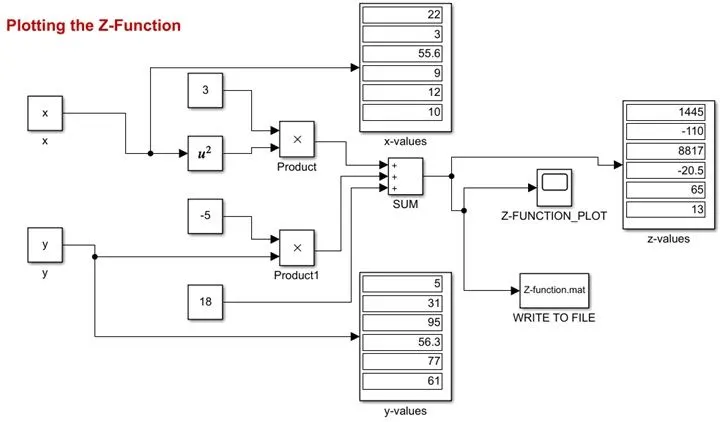
Figure 2 – Simulink model to calculate the polynomial function
(c) Mass-Spring Damper System:
In an effort to understand the mass-spring damper system, the Simulink and Simscape blocks are studied thoroughly. A basic schematic of the system is shown in Figure-3.
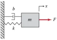
Figure 3 – Basic mass-spring damper system [Ref: chegg.com]
b – viscous damping coefficient [Ns2/m]
k - spring stiffness coefficient [N/m]
m – mass [kg]
F – excitation force [N]
x – displacement [m]
The Simulink and Simscape model of the mass-spring damper system is shown in Figure 4. It is inferred that there is a damping coefficient [‘b’] and a spring stiffness force [‘k’] which are summed up and set equal to the forces on the right side of the equation. Depending on the value the force experienced by the system, the spring undergoes a certain displacement. The vibration is absorbed by a damper, usually a piston moving in a viscous fluid. For example in an automobile suspension system, the shock-absorber is attached to the chassis of the vehicle which acts as a damper to reduce the vibrations experienced by the chassis and hence by the passengers.
The governing equation for the mass-spring damper system is based on Newton’s second law of motion as given below:
`mx ̈+bx ̇+kx=F` Eqn. [4]
For a free vibration system,
We have F = `0`, which implies
`bx ̇+kx= -mx ̈` Eqn. [5]
Where,
b – damping coefficient [Ns2/m]
k - spring stiffness [N/m]
m – mass [kg]
F – excitation force [N]
x – displacement [m]
According to Newton’s second law of motion, we have,
F = ma Eqn. [6]
Thus the governing equation for the spring-mass damper system is given as,
(1/m)*[-kx –bv] = a Eqn. [7]
Where,
a – acceleration of the mass [m/s2]
v – mass velocity [m/s]
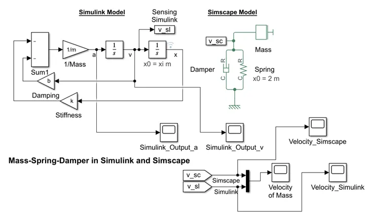
Figure 4 – Simulink and Simscape model of mass-spring damper system
RESULTS AND DISCUSSION
Part-I: Work done by the cutting tool in a shaping machine
The result for the work done (calculated by Eqn. [2]) is shown in Figure 5 and Table 1. It is noted from Table-1 that as the cutting length increases, the work done by the cutting tool also increases. This is mainly due to the surface area in contact with the cutting tool. At higher cutting depths, more work (or energy) is required to overcome the resistance of the material. Hence the increasing values of the tool work shown in Table-1.
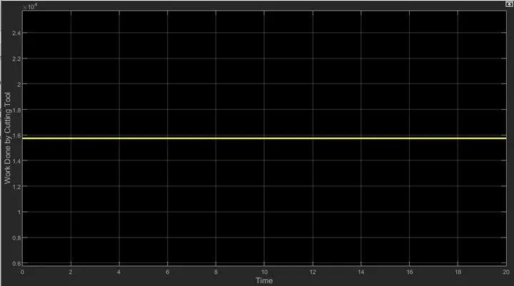
Figure 5 – Work done by Cutting tool in a shaping machine
|
Force [kN] |
Displacement [m] |
Work done [kJ] |
|
60 |
0 |
0 |
|
72 |
0.02 |
1.44 |
|
65 |
0.04 |
2.6 |
|
53 |
0.06 |
3.18 |
|
44 |
0.08 |
3.52 |
|
50 |
0.1 |
5 |
|
Total Work done |
15.74 kJ |
|
Table 1 – Calculation of Work done by Cutting tool in a shaping machine
(b) Plotting the Polynomial:
After calculating the coefficients of the polynomial, the sum of the various terms is used to arrive at the Z-function value (from Eqn. [3]). The polynomial coefficients are then written out to a “.mat” file which can later be opened in Matlab to view the polynomial coefficients. Figure 5 shows the polynomial function. It is noted from Figure 5 that the slope of the polynomial changes significantly around x=12 and after that the slope remains nearly constant.
In reality, the z-function can be used for to calculate a specific quantity based on the inputs provided or even extrapolate a value using an appropriate curve fit. For example, the thermal efficiency of an internal combustion engine vs pressure ratio can be plotted with empirical data and the curve can be used to extrapolate the thermal efficiency to larger pressure ratios.
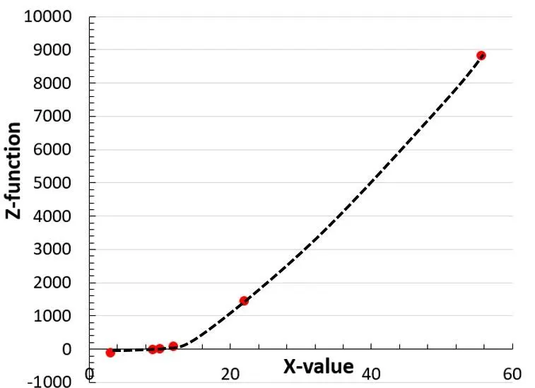
Figure 5 – Plot of polynomial function
(c) Response of Mass-Spring Damper System
(i) Effect of initial displacement on mass velocity and acceleration:
The time-dependent response of the mass-spring damper system is shown in Figures 6-19 for different initial displacement, mass, spring constant and damping coefficient. For an initial displacement (x0) of 1m, it is inferred from Figure 6 that the response signal is asymmetric about the horizontal axis for the Simulink case. The amplitude is higher on the negative side of the response compared to the positive side. It is also noted that the decay time of the response is approximately 3.5 seconds. The response from the Simscape signal (Figure 7) looks very similar to the Simulink variant. This confirms that the underlying mathematics and physics between Simulink and Simscape are identical for this problem.
When the initial displacement is increased to 2m, there is a significant increase in the signal response, as seen in Figure 8,9. Quantitatively, the difference in the signal amplitude is approximately twice the value at x0 = 1m. This can be attributed to the change in the initial displacement. On the other hand, the decay rate is steeper for the x0=2m case. It is also observed that the decay trend is similar to an exponential curve.
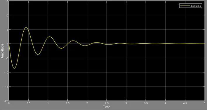
Figure 6 – Simulink velocity plot for x0=1;k=400;b=10;m=3.6
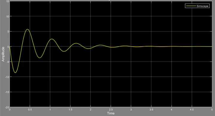
Figure 7 – Simscape velocity plot for x0=1;k=400;b=10;m=3.6
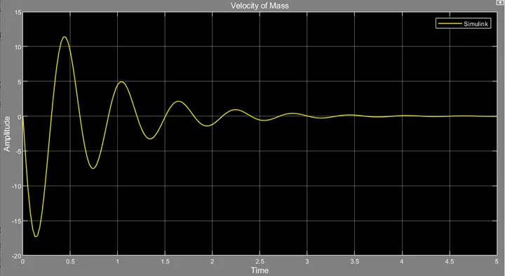
Figure 8 – Simulink velocity plot for x0=2;k=400;b=10;m=3.6
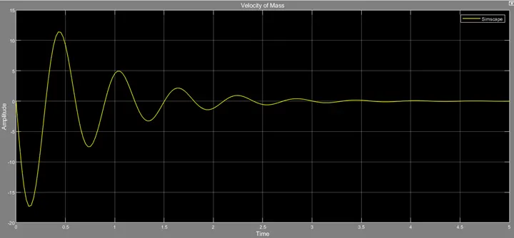
Figure 9 – Simscape velocity plot for x0=2;k=400;b=10;m=3.6
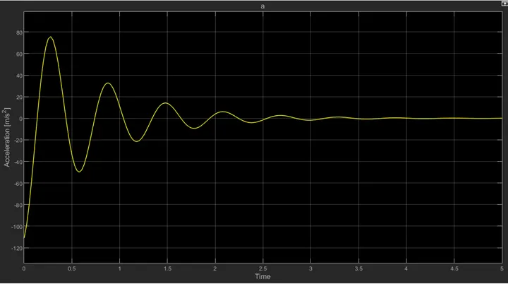
Figure 10 – Simulink acceleration plot for x0=1;k=400;b=10;m=3.6
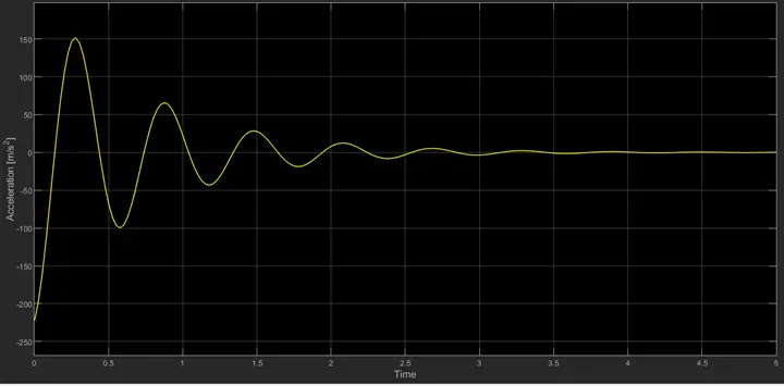
Figure 11 – Simulink acceleration plot for x0=2;k=400;b=10;m=3.6
ii) Effect of damping coefficient on the acceleration:
It is observed from Figures 12 and 13 that the damping coefficient reduces the decay time of the signal from 3.5 to 1.6 seconds approximately for x`0`=1 case. In addition, the maximum (positive) amplitude of the signal decreases from 77 to 55 m/s2 approximately. In the case of x`0`=2 (Figures 13 and 14), there is a reduction of 50 m/s2 (approximately) in the maximum positive acceleration when the damping coefficient is doubled. In addition, the signal decay time drastically reduces from 3.5 seconds to 1.8 seconds.
Figure 12 – Simulink acceleration plot for x0=1;k=400;b=10
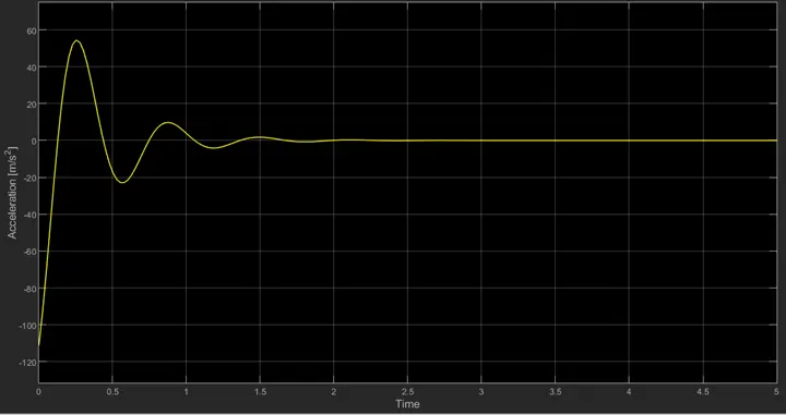
Figure 13 – Simulink acceleration plot for x0=1;k=400;b=20
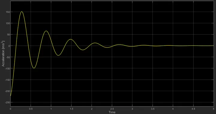
Figure 14 – Simulink acceleration plot for x0=2;k=400;b=10;m=3.6
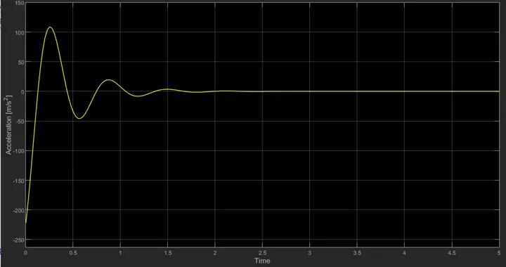
Figure 15 – Simulink acceleration plot for x0=2;k=400;b=20;m=3.6
iii) Effect of spring stiffness on the acceleration:
The effect of spring stiffness on the mass acceleration is shown in Figures 16,17. As the stiffness of the spring is increased, the acceleration of the mass reduces since the initial displacement is constant. The reduction in the maximum (positive) acceleration is approximately 30 m/s2. However, the decay rate of the signal remains nearly unchanged. This could be due to the same damping coefficient.
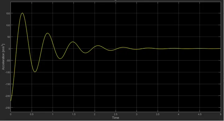
Figure 16 – Simulink acceleration plot for x0=1;k=400;b=10;m=3.6
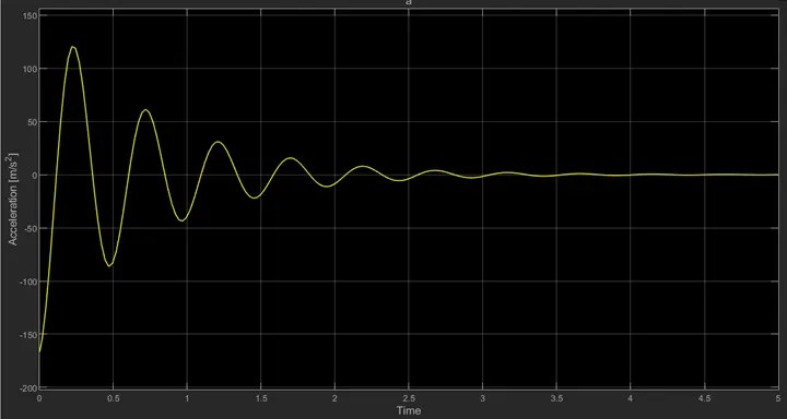
Figure 17 – Simulink acceleration plot for x0=1;k=600;b=10;m=3.6
v) Effect of body mass on the acceleration:
The effect of body mass on the acceleration in the case of Simulink is shown in Figures 18 and 19. It is inferred that the maximum (positive) acceleration decreases by approximately 29 m/s2 when the mass is increased from 3.6 kg to 7.2 kg. One reason for this could be the moment of inertia of the heavier mass, which moves at a slower velocity for the same initial displacement. In addition, the decay time of the signal has almost doubled. This indicates that the mas value has a direct impact on the decay time of the signal.
In Simscape, while attempting to change the value of mass in the Simscape source code, the access to change the mass value was denied. This is likely to be the default value in the Simscape block which is locked for editing.
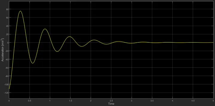
Figure 18 – Simulink acceleration plot for x0=1;k=400;b=10;m=3.6
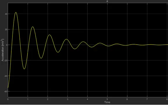
Figure 19 – Simulink acceleration plot for x0=1;k=400;b=10;m=7.2
CONCLUSIONS
In this project, the focus was to understand the usage of Simulink and Simscape blocks for problems involving mathematical and physical constraints. In addition, governing equations were derived for two of the problems using inference from the block diagram. The array multiplication block was well understood and was used in beneficially in two of the solutions as part of the challenge. The difference in the signal response when the body mass, spring stiffness and the damping coefficient were changed was interesting. Relevant observations were recorded and presented in the above sections appropriately. In summary, this project helped to get deeper understanding of the mathematical models associated with a problem.
REFERENCES
- https://nptel.ac.in/content/storage2/courses/112103022/module1/lec1/7.html
- Matlab R2020b Documentation, Mathworks Inc.
***************************End of Project*******************************