Simulation of the Harmonic Motion of a Simple Pendulum

Aim:

Ordinary differential equations are used to model several real life applications. Some of the applications include Fluid Mechanics, Heat Transfer, Vehicle Dynamics, Vibrations, Aero-Acoustics, Flow-induced Vibrations, etc. In this challenge, the harmonic motion of a Simple Pendulum is simulated in Matlab by solving a second order ordinary differential equation (ODE).

Schematic/Diagram:

A schematic of a Simple Pendulum is shown below.

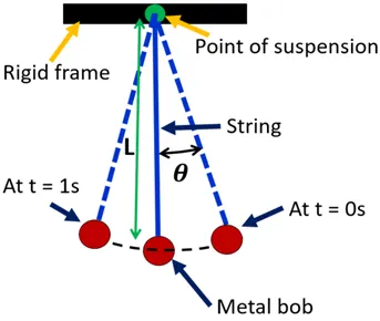
Figure 1 - Schematic of a Simple Pendulum

In Fig.1, it should be noted that,

`θ`– angular displacement [rad/s]

L – string length [m]

t – time period [sec]

Governing Equations:

The angular displacement as a function of time is expressed in the form of a second order ODE as follows:

`(d^2 θ)/dt^2 +(b/m)(dθ)/dt+g/L sinθ=0` Eqn. [1]

Where,

b – damping coefficient [-]

m – pendulum mass [kg]

g – acceleration due to gravity [m/s²]

L – string length [m]

t – time [sec]

`θ`– angular displacement [rad]

Since we are trying to solve the ODE using Matlab, we need to rewrite the second order ODE in the form of two first order ODEs. In order to do that, we set , `θ=θ_1`in Eqn. [1] and do the following:

`(dθ)/dt=(dθ_1)/dt=θ_2` Eqn. [2]

`(d^2 θ)/dt^2 =d/dt ((dθ_1)/dt)=(dθ_2)/dt=-(b/m θ_2+g/L sinθ_1 )` Eqn. [3]

In order to solve equations 2 and 3 in Matlab, we need to arrange them in a matrix format as shown below:

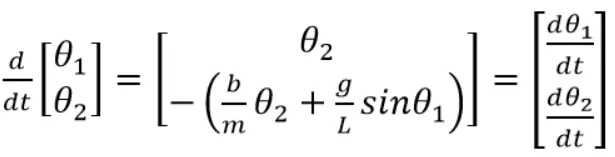Eqn. [4]

Where,

The left hand side of Eqn. [4] is the solution vector and the right hand side are the derivatives.

Using the initial condition of zero angular displacement and angular velocity = 3 rad/sec at time = 0 seconds, the ODE is solved using the ODE45 solver in Matlab.

The time period (T) for one complete oscillation i.e., one to and fro motion of the pendulum is analytically given by:

`T=2π*(L/g)^(1/2)` Eqn. [5]

Objective:

The main objective of this project is to understand and solve the governing equation to obtain the angular displacement and velocity for the harmonic motion of a simple pendulum. The solving of the ODE is performed in Matlab.

Main Content:

Program Algorithm for Main Code:

Main Code:

%-----------------Start of Program-----------------------
%Solving Second order ODE for Simple Pendulum harmonic motion 
%Code prepared by Srikrishna Mahadevan
%Clear and close all previous calculations, figures, etc.
clear all
close all
clc
%Inputs for the ODE
b = 0.05;%damping coefficient [-]
g = 9.81;%acceleration due to gravity [m/s^2]
L = 1;%length of the pendulum in [m]
m = 1;%mass of the pendulum in [kg]

%Initial condition 
theta_0 = [0;3];%zero initial displacement;3 rad/s angular velocity

%Time steps and total time
time_span = linspace(0,20,300);%total time of 20 seconds

%Solving the ODE using Matlab ODE45 solver
%ode_function is a function that is called here to rearrange the governing
%equation in a specific format for Matlab's ODE45 solver
[time, results] = ode45(@(time,theta) ode_function(time,theta,b,g,L,m),time_span,theta_0);

%Calculating the pendulum displacement with time
%for loop for calculating the pendulum displacement at 
%various time instants
ct=1;%initializing the figure count
tic %start the timer before for loop execution
for i = 1:length(time_span)%for loop definition
    THETA = results(i,1);%assigning value for angular displacement
x0 = 2;%x coordinate at the point of suspension of string
y0 = 2;%y coordinate at the point of suspension of string
x1 = x0+L*sin(THETA);%x coordinate at the end of the string
y1 = y0-L*cos(THETA);%y coordinate at the end of the string
%Plotting the simple pendulum displacement in real time
figure(ct)%setting the figure count
%plotting the string location
plot([x0 x1],[y0 y1],'blue','linewidth',6);
title('Simple Pendulum Simulation');%providing plot title
set(gca,'fontsize', 20);%providing plot text size
hold on
%plotting the rigid location where the pendulum is suspended
plot([1 3],[2 2],'black','linewidth',10);
%plotting the point of suspension of the pendulum
plot(x0, y0,'o','color','green','linewidth',5);
%plotting the pendulum mass
plot(x1, y1,'o','color','red','linewidth',20);
%providing labels for the x and y axis
xlabel('x-position [m]')
ylabel('y-position [m]')
%setting the axis limits
axis([0 4 0.5 2])
%enabling the grid display
grid on
grid minor
pause(0.3)%pausing the code execution to view the pendulum location
%get individual frames from the current figure window
M(ct) = getframe(gcf);
ct = ct+1;%counter to increment figure
end %end the for loop
toc %calculate and display the total time for loop execution
%Creating Movie from the individual frames
movie(M)
% %Creating a ".avi" format of the movie to play it in Media player
videofile = VideoWriter('Simple_Pendulum_Srikrishna.avi','Uncompressed AVI');
% %Open the video file, copy the individual frames into it,
% % and close the file
open(videofile)
writeVideo(videofile,M)
close(videofile)

%Plotting the angular displacement and velocity of the 
%Simple Pendulum vs time
figure(301)%assigning the figure number
%Plotting the angular displacement vs time
plot(time,results(:,1),'color','blue','linewidth',3)
set(gca,'fontsize', 20);%setting the text font size
hold on %holding on the plot for including more data
%Plotting the angular velocity vs time
plot(time,results(:,2),'color','red','linewidth',3)
title('Simple Pendulum Displacement and Velocity');%providing the plot title
%Defining the plot legend
legend('Displacement','Velocity');
%Including the axis labels
xlabel('Time [seconds]')
ylabel('Displacement [rad],Velocity [rad/s]')
%enabling the grid display
grid on
grid minor

%Calculating the oscillation time period (T) of the simple pendulum for 
%a fixed string length of '1m'
T = 2*pi()*(L/g)^0.5 %printing out the time period
%Calculating the oscillation time period (T) of the simple pendulum for 
%multiple string lengths 
L1 = linspace(0.1,10,50);%defining the string length array
T1 = 2*pi()*(L1./g).^0.5;%calculating the time period
%Plotting the time period vs string length
figure(302)%assigning the figure number
%plotting the time period for multiple string lengths
plot(L1, T1,'blue','linewidth',4);
title('Simple Pendulum Time Period');%providing the plot title
set(gca,'fontsize', 20);%specifying the text font size
hold on
%plotting the time period for L = 1m on the same plot
plot(L, T,'o','color','red','linewidth',8);
%providing labels for the x and y axis
xlabel('String Length [m]')
ylabel('Time Period of Oscillation [sec]')
% axis([0 10 0 30])
%enabling the grid display
grid on
grid minor

% -----------------------End of program------------------------------

Program Algorithm for ODE Function Code:

ODE Function Code:

%Function to express the higher order ODEs in the form of multiple first order ODE
%terms --> easier to integrate and solve; function takes input values for 
function[dtheta_dt] = ode_function(time,theta,b,g,L,m)%function definition
theta1 = theta(1);%assigning the first term in the solution matrix
theta2 = theta(2);%assigning the second term in the solution matrix
dtheta1_dt = theta2;%expressing the first derivative in terms of 
% a new variable theta2
%Expressing the governing equation in terms of new variables
dtheta2_dt = -(b/m)*theta2 - (g/L)*sin(theta1);
%writing the equation for the solution matrix 
dtheta_dt = [dtheta1_dt; dtheta2_dt];
end %end of function

Results and Discussion:

The angular displacement and velocity for multiple damping coefficients are shown in Figure 2. As a general observation, the angular displacement and velocity exhibit a sinusoidal pattern as they decay with increase in time. It is inferred from Fig. 2a that the decay in the angular displacement and velocity is very gradual since the damping coefficient is a very small value [b=0.05]. But as we increase the damping coefficient to 0.225 in Fig. 2b, we can see that the decay is more significant. For the highest damping coefficient [b=0.5], the exponential decay is evident from Fig. 2c.

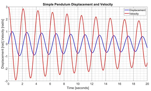
Figure 2a - Angular Displacement and Velocity for b = 0.05

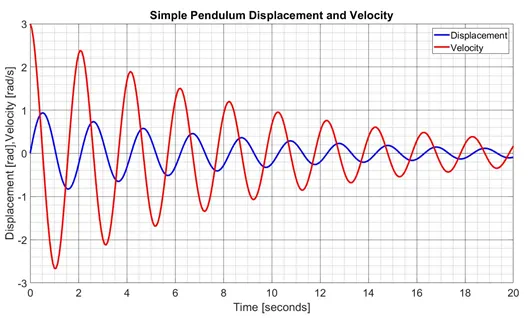
Figure 2b - Angular Displacement and Velocity for b = 0.225

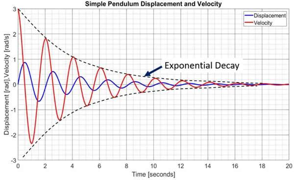
Figure 2c - Angular Displacement and Velocity for b = 0.5

By plotting the Time period of oscillation (T) for multiple string lengths in Fig. 3, it can be observed that there is an exponential increase in the Time period of oscillation as the string length is increased. This is because the moment of inertia of the system has reduced which reduces the angular velocity. On the other hand, short strings have higher moment of inertia enabling them to return to their start position quicker. The Time period of oscillation (T) for L = 1m in shown by the red marker in Fig. 3.

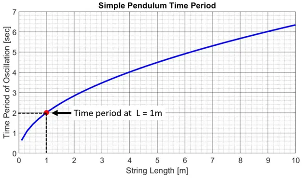
Figure 3 – Time Period of Oscillation for multiple string lengths

Animation of Simple Pendulum Motion:

An animated video of the harmonic motion of the Simple Pendulum can be viewed by clicking on the following link:

https://drive.google.com/file/d/1IQ1I9oBu3zd-PZQZL1QGA9_EHyNZMHQ-/view?usp=sharing

It can be observed from the animation that the simple pendulum exhibits an oscillating motion with time. With increase in time, the displacement and velocity decrease according to the governing equation. If the pendulum mass is increased, the decay will be much faster for the same velocity and string length.

Conclusions:

The simple pendulum project enables us to understand the working principle of a simple harmonic oscillator and its governing equation. In addition, we could see the influence of the damping coefficient and string length on the angular displacement, velocity and the time period of oscillation. As an additional effort, we could investigate the pendulum motion (animation) for multiple masses and string lengths. The knowledge gained from this project can be utilized to study more complex real world applications.