Basics of Simulink

Introduction:

Often times in today’s digital world, it is needed to simulate a system, sub-system or a small component using a virtual setup which has mathematical and physical resemblance with the actual application. Obviously, conducting a reliable experiment is the ideal procedure to achieve the goal. Due to time and resource constraints, it is advisable to perform essential back of the envelope calculations before moving ahead to the final design parameters. Simulink provides a platform to virtually test a system, understand and interpret its functionality and identify the scope for improvement. Simulink emphasizes on the correct logic, robustness, simplicity, etc. of the model.

Aim:

The aim of this project is a two-fold as given below:

1. To generate a mathematical function using the provided equation in Simulink and plot the function.
2. To run an existing Simulink program called “Suspension System Comparison” and describe its objectives, working and observations from the results.

Objectives:

The main objectives of this project include (i) understanding the function of the basic Simulink blocks (ii) Compare the different suspension systems and explain the similarities/differences (iii) detail the observations from the results (iv) explain the creation of an oscillating velocity source

Governing Equations:

The force exerted by a linear spring is given as,

F = K*x Eqn.[1]

In the case of a damper, the damping force F_D is given as,

F_D = B*v Eqn.[2]

The force exerted by a non-linear spring is given as,

`F=k_1 x+sign(x)*k_2 x^2+k_3 x^3+sign(x)*k_4 x^4+k_5 x^5 Eqn.[3]`

Relative displacement between ports R and C is given as,

`x=x_i+x_R-x_C`

where:

F –spring force

K – Spring stiffness [N/m]

B - damping coefficient [N/(m/s)]

v – relative velocity between ports ‘R’ and ‘C’ [rad/s]

k₁, k₂, …....., k_n — Spring coefficients

x — Relative displacement between ports R and C

x_i — Initial relative displacement

x_R— Absolute displacement associated with port R

x_C — Absolute displacement associated with port C

At simulation start (t=0), x_R and x_C are zero. The corresponding x_init is then calculated.

Results and Discussion:

(i) Plot a function y(x) = (x-1) * (x-3)^2 * (x-9)^2 using basic Simulink blocks.

In order to plot the above function in Simulink, the function was split into 3 terms as shown below:

Term-1 : [x-1]

Term-2 : [x-3]²

Term-3 : [x-9]²

After evaluating the terms separately, the product of the terms is calculated using the Product block. The Simulink code can be found in the link below.

Part (i) Simulink code link

https://drive.google.com/drive/folders/1-EaYdSmu8o8Uzl2JyABJ36eFZdMd2-US?usp=sharing

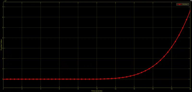
Figure 1 – Plot of the mathematical function

The function plot shows a nearly constant line until time = 11 seconds, after which there is a gradual (non-linear) increase in the function output. It should be noted here that only the variation in the function output is relatively small in Initial and boundary conditions are specified based on the block.

Objectives of the Suspension system comparison program:

The main objectives of this program include:

1. To understand the physics and mathematics of an automobile suspension system modeled in Simulink
2. To compare the different suspension systems and identify the similarities/differences
3. To replicate the existing Simulink program and gain insight into the results

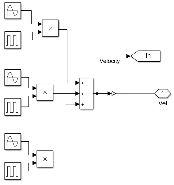
Figure 2a – Velocity input block diagram for the suspension system

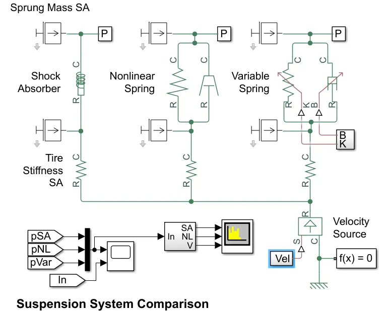
Figure 2b – Block diagram for the suspension system comparison

A combination of the sinusoidal waveform block in used in conjunction with a pulse generator block and the product of the two blocks is summed up along with the other sinusoidal waveforms (with time and phase lag) to get the final input signal. It should be noted that the frequency of the three signals are 3, 15 and 75Hz respectively.

Oscillating velocity source creation:

After observing the input signal (i.e. velocity and amplitude), it is inferred that the frequency of the three signals are 3, 15 and 75Hz respectively. The frequency of the signals differ by a multiplication factor of five. However, the signal amplitude remains the same across the three signals (for the sinusoidal waveform) with no bias or phase difference.

In order to generate the velocity source, a combination of the sinusoidal waveform block in used in conjunction with a pulse generator block and the product of the two blocks is summed up along with the other two sinusoidal waveforms (with time and phase lag) to get the final input signal. In the final input signal, there is a relative time lag of 20 seconds between the three signals. In addition, there is a phase delay of 40 seconds between the different pulses in the pulse generator block.

Spring-mass damper system:

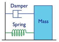
Figure 3 – Spring mass damper system [1]

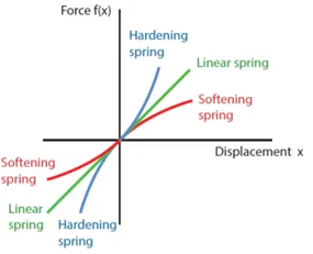
Figure 4 – Typical Force vs displacement curves for linear and non-linear springs [1]

The different damping systems used in the suspension system are,

1. Shock absorber

2. Non-linear spring

3. Variable spring

Shock absorber:

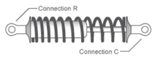
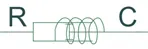
Figure 5 – Shock absorber schematic and simulink block

A shock absorber is a spring-damper system, which is used to dampen vibration in mechanical and electro-mechanical systems. In the case of translational shock absorber, the initial spring force is zero if the initial deformation is set to zero. The total force between R and C is the sum of spring stiffness, damping, Coulomb friction and contributions from the hard stop configuration. The point ‘R’ is fixed to a rigid frame while ‘C’ moves based on the translational velocity. The sum of viscous and Coulomb friction provides the damping force. It is also possible to include hard stops that limit the spring-damper travel distance.

Non-linear spring

A non-linear translational spring has a nonlinear force-displacement curve. The spring force magnitude is a generic function of displacement. It is not required to satisfy the Hooke’s law. If the stiffness increases with increasing applied force, it is called a softening spring and if the displacement decreases with applied force, it is referred to as a hardening spring. The spring force can be symmetric or asymmetric with respect to zero deformation. By using polynomial and table lookup parameterizations, the force-displacement relationship can be specified. The spring force can be symmetric or asymmetric with respect to the initial deformation.

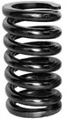
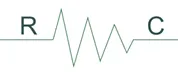
Figure 5 – Non-linear spring schematic and simulink block

Variable spring:

A linear variable spring is used when the spring stiffness needs to be adjusted. The spring force is calculated based on Eqn. [y]. It should be noted here that there is a lower threshold for the spring stiffness (K=1 N/m) avoids undesirable values for ‘K’. The force is taken to be positive when it acts from port R to port C.

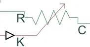
Figure 6 – Variable spring simulink block

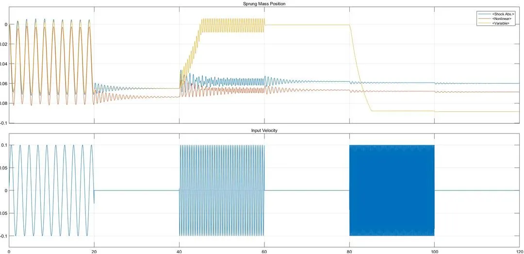
Figure 7 – Input velocity and spring mass position for the three suspension systems

Similarities:

1. All the three systems have a spring-mass damper configuration
2. The velocity source is identical between the different systems
3. The tire stiffness is identical between the different systems
4. A sprung mass is present in all the three systems

Differences:

1. The spring force vs displacement obeys Hooke’s law for the shock absorber but not necessarily for the other two systems
2. The spring stiffness is constant for the shock absorber; but, it can be varied in the case of variable spring
3. In the velocity source, there is a phase delay of 40 seconds between the different pulses

Conclusions:

In this project, a basic mathematical function was calculated and plotted using Simulink. In addition, the similarities and differences between three spring mass damper systems were studied in detail. Particularly, the input velocity signal was given more emphasis. Using the knowledge gained from this project, one can feel confident to build more complex programs in Simulink.

References:

1. Srinivasan, M., 2016, Non-linear dynamics lecture, Oklahoma State University.

2. Matlab Documentation, 2020, The MathWorks Inc.