File Parsing for NASA's Thermodynamic Data

Introduction:

In many industries and research laboratories, it is often needed to exchange information between different departments. In some cases, testing may be conducted in a different location and the back end team could be asked to read and interpret the data. In such situations, parsing the data is essential to extract only relevant information, which can be used for further analysis. Therefore, file parsing is a very important procedure to learn and understand.

Aim:

The primary goal of this project is to parse one of NASA’s thermodynamic data set, which contains polynomial coefficients for calculation of specific heat at constant pressure, enthalpy and entropy. In addition, the molecular weight of all the species is calculated.

Objectives:

The main objectives of this project are to (i) learn the underlying procedure of the file parsing (ii) write a Matlab code to parse a Thermodynamic data file from NASA (iii) Run the file parsing code for multiple species (i.e. chemical compounds) provided in the Thermodynamic data file (iv) Calculate the Cp, enthalpy and entropy for the different temperature ranges (v) Interpret the results for O2, N2 and CO2 species (vi) Automatically save the plots in appropriate species folders

Governing Equations:

The main governing equations used in this report are given below for the calculation of Specific heat at constant pressure (`C_p` ), enthalpy (h) and entropy (s).

`C_p/R=a1+[a2*T]+[a3*T^2 ]+[a4*T^3 ]+[a5*T^4 ]` Eqn. [1]

`h/(RT)=a1+[a2*T/2]+[a3*T^2/3]+[a4*T^3/4]+[a5*T^4/5]+[a6/T]` Eqn. [2]

`s/R=[a1*log⁡(T)]+[a2*T]+[a3*T^2/2]+[a4*T^3/3]+[a5*T^4/4]+a7` Eqn. [3]

where, 'R' is the universal gas constant with a value of 8.314 J/mol.K and 'T' is the species temperature in Kelvin.

It should be noted that the above equations contain the high temperature coefficients, which are used between middle and high local temperature range of a given species. If we need to use Eqns. [1-3] for the low temperature range, it is required to use the low temperature coefficients (a8 – a14) instead of a1-a7.

Main Content:

A Matlab code is written to read the NASA Thermodynamic Data file and read it in segments, such as comment lines, headers, species name, temperature ranges and polynomial coefficients. Once the polynomial coefficients are obtained, Cp, h and s are calculated and plotted versus the temperature values. Comments are provided at each step of the code to explain the command. The program algorithm and the code are given below. The code logic is described at a later part of this report.

Program Algorithm:

Line no.	Explanation
1	Comment Line
2	Comment Line
3	Comment Line
4	Comment Line
5	Clear all data
6	Close all data
7	Clear command window
8	Comment line
9	Reading NASA Thermo data file
10	getting the values of first line
11	getting the values of second line
12	saving the string data in variable 'title'
13	splitting the string data
14	Comment line
15	Comment line
16	Calculating the low, mid and high temp,Converting string to numerical data
17	Converting string to numerical data
18	Converting string to numerical data
19	Comment line
20	stepping through the comment lines using For loop
21	stepping through the comment lines
22	ending the for loop
23	Comment line
24	Defining the universal gas constant in kJ/mol.K
25	Comment line
26	Comment line
27	Comment line
28	Comment line
29	Comment line
30	Comment line
31	Using a for loop to read the species name for all species
32	index to the species header line
33	storing the species name data
34	splitting the species name data
35	Comment line
36	Reading the species name
37	Testing individual species name - Use this for user specific input of Species name;While using this line, diasble the main for loop (Line 31)
38	Comment line
39	Comment line
40	Defining Symbol of main elements
41	Comment line
42	Comment line
43	Defining Atomic weight of main elements
44	Comment line
45	Initializing the molecular weight
46	For loop for stepping through the Species_name
47	Comment line
48	For loop for stepping through the Elements
49	Comment line
50	If condition to compare the string name with the main elements
51	Calculating the Molecular weight for individual elements
52	storing the location of the element
53	else statement
54	ending the if statement
55	ending the second for loop
56	Converting the species name to num format
57	checking if N > 1
58	Calculating the Molecular weight for repeating elements
59	else statement
60	ending the if statement
61	ending the first for loop
62	Comment line
63	displaying the Molecular weight in the command window
64	displaying the units
65	Comment line
66	Comment line
67	Comment line
68	Comment line
69	Extracting the Local temperature range according to the species; calculating the low temp. value
70	calculating the high temp. value
71	calculating the mid temp. value
72
73	Comment line
74	Move to the next line to extract the first set of coefficients (1-5)
75	storing the species data
76	checking for 'E' in the species data
77	Comment line
78	capturing the 3 digits after exponent for the coefficient for A1
79	capturing the 3 digits after exponent for the coefficient for A2
80	capturing the 3 digits after exponent for the coefficient for A3
81	capturing the 3 digits after exponent for the coefficient for A4
82	capturing the 3 digits after exponent for the coefficient for A5
83	Comment line
84	converting string to double data for A1
85	converting string to double data for A2
86	converting string to double data for A3
87	converting string to double data for A4
88	converting string to double data for A5
89	Comment line
90	Move to the next line to extract the second set of coefficients (6-10)
91	storing the species data
92	checking for 'E' in the species data
93	Comment line
94	capturing the 3 digits after exponent for the coefficient for A6
95	capturing the 3 digits after exponent for the coefficient for A7
96	capturing the 3 digits after exponent for the coefficient for A8
97	capturing the 3 digits after exponent for the coefficient for A9
98	capturing the 3 digits after exponent for the coefficient for A10
99	Comment line
100	converting string to double data for A6
101	converting string to double data for A7
102	converting string to double data for A8
103	converting string to double data for A9
104	converting string to double data for A10
105
106	Comment line
107	Move to the next line to extract the third set of coefficients (11-14)
108	storing the species data
109	checking for 'E' in the species data
110	Comment line
111	capturing the 3 digits after exponent for the coefficient for A11
112	capturing the 3 digits after exponent for the coefficient for A12
113	capturing the 3 digits after exponent for the coefficient for A13
114	capturing the 3 digits after exponent for the coefficient for A14
115	Comment line
116	converting string to double data for A11
117	converting string to double data for A12
118	converting string to double data for A13
119	converting string to double data for A14
120	Comment line
121	Comment line
122	X-axis data for temperature
123	Comment line
124	Initialising the value for Cp
125	Initialising the value for h
126	Initialising the value for s
127	Comment line
128	Initializing for loop for temperature range
129	Comment line
130	Comment line
131	checking the if condition for the low temperature range
132	Comment line
133	Comment line
134	calculating Cp for the low temperature range
135	Comment line
136	calculating h for the low temperature range
137	Comment line
138	calculating s for the low temperature range
139	else statement
140	Comment line
141	Comment line
142	calculating Cp for the high temperature range
143	Comment line
144	calculating h for the high temperature range
145	Comment line
146	calculating s for the high temperature range
147	ending the if else statement
148	ending the for loop
149
150	Comment line
151	Comment line
152	setting the figure properties for Cp plot
153	plotting the Cp values vs temperature
154	providing plot title
155	providing plot text size
156	providing the x-label
157	providing the y-label
158	Comment line
159	Comment line
160	switching on the axis grid
161	switching on the axis minor grid
162
163	Comment line
164	Creating a folder to save the plot images
165	Comment line
166	going into the folder of the corresponding species
167	Comment line
168	Saving the Cp plot
169
170	Comment line
171	setting the figure properties for h plot
172	plotting the Cp values vs temperature
173	providing plot title
174	providing plot text size
175	providing the x-label
176	providing the y-label
177	Comment line
178	Comment line
179	switching on the axis grid
180	switching on the axis minor grid
181	Comment line
182	Saving the h plot
183
184	Comment line
185	setting the figure properties for h plot
186	plotting the s values vs temperature
187	providing plot title
188	providing plot text size
189	providing the x-label
190	providing the y-label
191	Comment line
192	Comment line
193	switching on the axis grid
194	switching on the axis minor grid
195	Comment line
196	Saving the s plot
197	going back to the parent folder
198	end the for loop
199	Comment line

Matlab Program:

%-----------------Start of Program-----------------------
%File Parsing Using MATLAB
%Code prepared by Srikrishna Mahadevan
%Clear and close all previous calculations, figures, etc.
clear all
close all
clc
%Reading NASA Thermo data file
fnasa = fopen('THERMO.dat','r');
H1 = fgetl(fnasa);%getting the values of first line
H2 = fgetl(fnasa);%getting the values of second line
tline = H2;%saving the string data in variable 'title'
H2 = strsplit(tline, ' ');%splitting the string data
%Converting string to numerical data
%Calculating the low, mid and high temp
global_low_temp_value = str2double(H2{2});%low temp
global_mid_temp_value = str2double(H2{3});%mid temp
global_high_temp_value = str2double(H2{4});%high temp
%stepping through the comment lines using For loop
for i = 1:3
    fgetl(fnasa);%stepping through the comment lines
end
% Defining the universal gas constant in kJ/mol.K
R = (8.314/1000);
%Writing the Molecular weight to a text file
% MW = fopen('molecular_weight.txt','w');
% fprintf(MW,'%16s %16sn','Species','Molar Mass');
%Using a for loop to read the species name for all species
%Using a second for loop to index through the relevant 
%Periodic table elements
for j=1:3 %for loop definition
    species_H = fgetl(fnasa);%index to the species header line
    tline = species_H;%storing the species name data
    species_H = strsplit(tline, ' ');%splitting the species name data
    %Extracting the species name and displaying in command window
    Species_name = species_H{1}
    %Species_name = 'H2O'% Testing individual species name
    %Calculate the molecular weight of the species 
    %Defining Symbol of main elements
    Elements = ["C";"H";"O";"N";"Ar"];
    %C-Carbon ; H-Hydrogen; O-Oxygen; N-Nitrogen; Ar-Argon
    %Defining Atomic weight of main elements
    At_weights = [12.01;1.008;16;14.06;39.95];
    %For loop for stepping through the Species_name
    Molecular_weight = 0;%Initializing the molecular weight
    for m = 1:length(Species_name)
          %For loop for stepping through the Elements
        for n = 1:length(Elements)
        %If condition to compare the string name with the main elements
            if (strcmpi(Species_name(m),Elements(n)) == 1)
                Molecular_weight = Molecular_weight + At_weights(n);
                location = n;
            else
            end
        end
            N = str2num(Species_name(m));
            if (N > 1)
                Molecular_weight = Molecular_weight + (At_weights(location)*(N-1));
            else
            end
    end
    %Calculating the total Molecular Weight
    Molecular_weight_Species = Molecular_weight
    Units = 'g/mol'
%     %Writing the Molecular weight to a text file
%     fprintf(MW,'%16.7f %16.7f',Species_name(m), Molecular_weight(m));
%     fprintf(MW,'n');
    % Extracting the Local temperature range according to the species
    Species_low_temp = str2double(species_H{length(species_H)-3});%Low temp
    Species_high_temp = str2double(species_H{length(species_H)-2});%High temp
    Species_mid_temp = str2double(species_H{length(species_H)-1});%Mid temp
   
    %Move to the next line to extract the first set of coefficients (1-5)
    species_H = fgetl(fnasa);%reading the species data
    tline = species_H;%storing the species data
    species_L1 = strfind(tline,'E');%checking for 'E' in the species data
    %capturing the 3 digits after exponent for the coefficient
    A1 = tline(1:species_L1(1)+3);
    A2 = tline(species_L1(1)+4:species_L1(2)+3);
    A3 = tline(species_L1(2)+4:species_L1(3)+3);
    A4 = tline(species_L1(3)+4:species_L1(4)+3);
    A5 = tline(species_L1(4)+4:species_L1(5)+3);
    %converting the coefficients into floating point number 
    A1 = str2double(A1);
    A2 = str2double(A2);
    A3 = str2double(A3);
    A4 = str2double(A4);
    A5 = str2double(A5);
    %Move to the next line to extract the first set of coefficients (6-10)
    species_H = fgetl(fnasa);%reading the species data
    tline = species_H;%storing the species data
    species_L2 = strfind(tline,'E');%checking for 'E' in the species data
    %capturing the 3 digits after exponent for the coefficient
    A6 = tline(1:species_L2(1)+3);
    A7 = tline(species_L2(1)+4:species_L2(2)+3);
    A8 = tline(species_L2(2)+4:species_L2(3)+3);
    A9 = tline(species_L2(3)+4:species_L2(4)+3);
    A10 = tline(species_L2(4)+4:species_L2(5)+3);
    %converting the coefficients into floating point number 
    A6 = str2double(A6);
    A7 = str2double(A7);
    A8 = str2double(A8);
    A9 = str2double(A9);
    A10 = str2double(A10);
    
  %Move to the next line to extract the third set of coefficients (11-14)
    species_H = fgetl(fnasa);%reading the species data
    tline = species_H;%storing the species data
    species_L3 = strfind(tline,'E');%checking for 'E' in the species data
    %capturing the 3 digits after exponent for the coefficient
    A11 = tline(1:species_L3(1)+3);
    A12 = tline(species_L3(1)+4:species_L3(2)+3);
    A13 = tline(species_L3(2)+4:species_L3(3)+3); 
    A14 = tline(species_L3(3)+4:species_L3(4)+3);
    %converting the coefficients into floating point number 
    A11 = str2double(A11);
    A12 = str2double(A12);
    A13 = str2double(A13);
    A14 = str2double(A14);
% Using the local temperature range for calculation of Cp, h ,s
%Defining temperature array
temp = linspace(Species_low_temp,Species_high_temp,500);%X-axis data for temperature
% temp = transpose(temp);
Cp = 0;%Initialising the value for Cp
h = 0;%Initialising the value for h
s = 0;%Initialising the value for s
%Initializing for loop for temperature range
for u = 1:length(temp)
    %Using if condition to switch between 
    %low and high temperature coefficients
    if (temp(u) <= Species_mid_temp)
%Calculating Cp using polynomial curve fit
%For Low temp data [Coefficients A8 to A14]
Cp(u) = R*(A8+(A9*temp(u))+(A10*temp(u)^2)+(A11*temp(u)^3)+(A12*temp(u)^4));
%Calculating enthalpy (h) using polynomial curve fit
h(u) = (R*temp(u))*(A8+(A9*(temp(u)/2))+(A10*(temp(u)^2/3))+(A11*(temp(u)^3/4))+(A12*(temp(u)^4/5))+(A13/temp(u)));
%Calculating entropy (s) using polynomial curve fit
s(u) = R*((A8*log(temp(u)))+(A9*temp(u))+(A10*(temp(u)^2/2))+(A11*(temp(u)^3/3))+(A12*(temp(u)^4/4))+A14);
    else
%Calculating Cp, H, S using polynomial curve fits - MID TEMP TO HIGH TEMP
%For High temp data [Coefficients A1 to A7]
Cp(u) = R*(A1+(A2*temp(u))+(A3*temp(u)^2)+(A4*temp(u)^3)+(A5*temp(u)^4));
%Calculating enthalpy (h) using polynomial curve fit
h(u) = (R*temp(u))*(A1+(A2*(temp(u)/2))+(A3*(temp(u)^2/3))+(A4*(temp(u)^3/4))+(A5*(temp(u)^4/5))+(A6/temp(u)));
%Calculating entropy (s) using polynomial curve fit
s(u) = R*((A1*log(temp(u)))+(A2*temp(u))+(A3*(temp(u)^2/2))+(A4*(temp(u)^3/3))+(A5*(temp(u)^4/4))+A7);
    end
end
    
%Plotting the variation of Cp, H, S with temperature
%setting the figure properties for Cp plot
figure('units','normalized','outerposition',[0 0 1 1])
plot(temp, Cp,'black','linewidth',4)%plotting the Cp values vs temperature
title('Specific Heat vs Temperature');%providing plot title
set(gca,'fontsize', 20);%providing plot text size
xlabel('Temperature [K]')%providing the x-label
ylabel('Specific Heat at Constant Pressure [kJ/kgK]')%providing the y-label
%setting the axis limits
% axis([0 0.6 0 0.6])
grid on %switching on the axis grid
grid minor %switching on the axis minor grid

%Creating a folder to save the plot images
mkdir(['C:UsersSriDocumentsMATLABFile_Parsing_Plots',Species_name]);
%going into the folder of the corresponding species
cd(['C:UsersSriDocumentsMATLABFile_Parsing_Plots',Species_name])
%Saving the Cp plot 
saveas(gcf,'Cp.jpg')

%setting the figure properties for h plot
figure('units','normalized','outerposition',[0 0 1 1])
plot(temp, h,'blue','linewidth',4)%plotting the h values vs temperature
title('Enthalpy vs Temperature');%providing plot title
set(gca,'fontsize', 20);%providing plot text size
xlabel('Temperature [K]')%providing the x-label
ylabel('Enthalpy [kJ/kg]')%providing the y-label
%setting the axis limits
% axis([0 0.6 0 0.6])
grid on %switching on the axis grid
grid minor %switching on the axis minor grid
%Saving the h plot 
saveas(gcf,'enthalpy.jpg')

%setting the figure properties for s plot
figure('units','normalized','outerposition',[0 0 1 1])
plot(temp, s,'red','linewidth',4)%plotting the s values vs temperature
title('Entropy vs Temperature');%providing plot title
set(gca,'fontsize', 20);%providing plot text size
xlabel('Temperature [K]')%providing the x-label
ylabel('Entropy [kJ/kg]')%providing the y-label
%setting the axis limits
% axis([0 0.6 0 0.6])
grid on %switching on the axis grid
grid minor %switching on the axis minor grid
%Saving the s plot 
saveas(gcf,'entropy.jpg')
cd 'C:UsersSriDocumentsMATLABFile_Parsing_Plots' %returning to the home directory
end %end the for loop
% ++++++++++++++++++++++++++++End of Program++++++++++++++++++++++++++++++++++++

Program Logic:

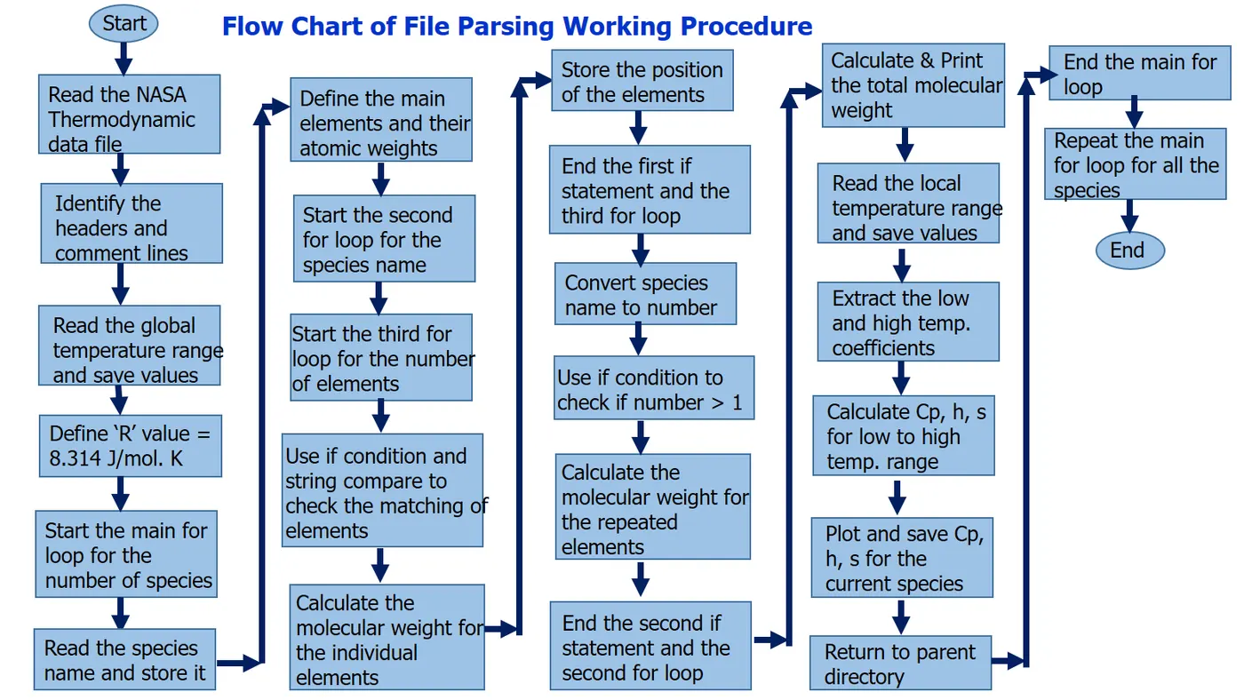
A simple block diagram is given below that explains the logic behind the Matlab code to parse the NASA data file.

Molecular Weight Calculation:

In order to calculate the molecular weight, the atomic weight of the main elements are used. In addition, if there are any repeating terms in the species name, they are accounted using the following logic.

Step:1 – Check the species name and compare the characters with the main elements (Table-1)

Step:2 – If the species name matches with the main elements, then the corresponding atomic weights are used

Step:3 – In the case of repeating elements, the number of repetitions is used to add the additional atomic weight to the individual elements to get the total value

Step:4 – Print the molecular weight to the command window

Step:5 – Increment the for loop to account for all the terms in the species name

Step:6 - Repeat the main for loop for all the species

Table 1 – Atomic weights and symbols of main elements

Element Symbol	Element Name	Atomic Weight [g/mol]
O	Oxygen	16
H	Hydrogen	1.008
C	Carbon	12.01
N	Nitrogen	14.01
Ar	Argon	39.95

User defined input:

If the user wants to enter a specific name for the species, it can be done via Line 37 of the Matlab code. While doing this, the main for loop (starting at Line 31) must be disabled so that the program can be executed only for the entered species name. The value of the polynomial coefficients must be specified directly for user defined input. This can be done by specifying values for coefficients a1,a2,a3,……….a14 directly in the code. In this case, the automated calculation of the coefficients can be disabled in the code.

Results and Discussion:

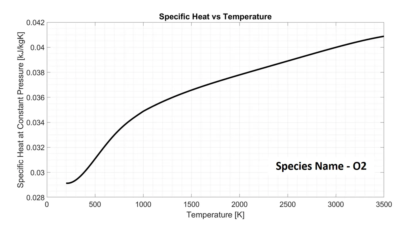
Figure 1a - Specific heat vs temperature for O2 species

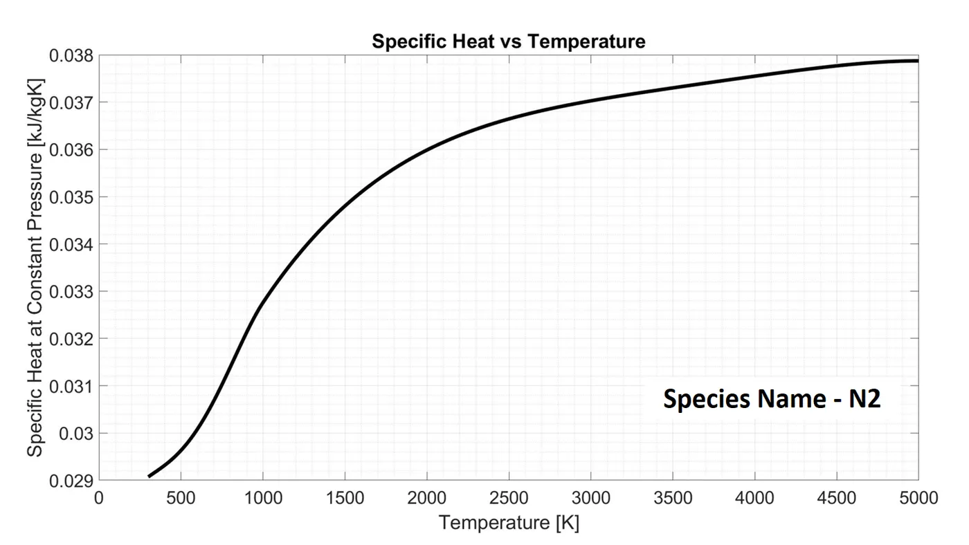
Figure 1b - Specific heat vs temperature for N2 species

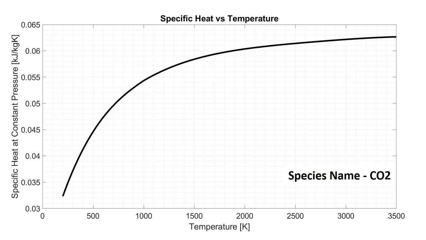
Figure 1c - Specific heat vs temperature for CO2 species

The `C_p` plots are shown in Fig. 1 for O2, N2 and CO2 species. It can be inferred from Fig. 1a that the trend in the `C_p` curve is non-linear till 400 K (approximately) after which it becomes close to linear with three different slopes. The first linear part is between 400 and 800 K, the second from 800 to 1000 K and the longer segment of the linear curve is between 1000 K and 3500 K. In Fig. 1b, the plot is shown for N2 species. The variation of `C_p` is close to a cubic fit between 200 and 2500 K, after which the trend becomes more towards a linear fit. In the case of CO2 species (Fig. 1c), the curve is similar to a bounded exponential growth profile, which asymptotes to a `C_p` value of 0.0625 kJ/kg K at higher temperatures.

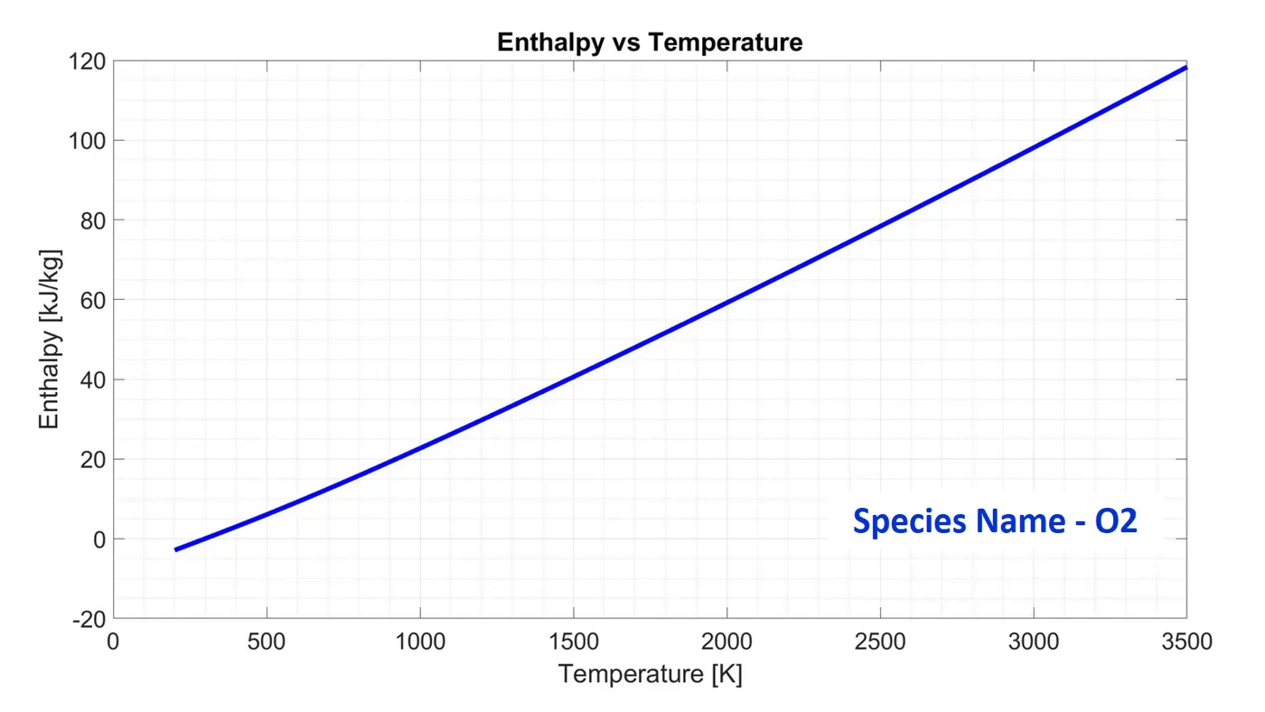
Figure 2a - Enthalpy vs temperature for O2 species

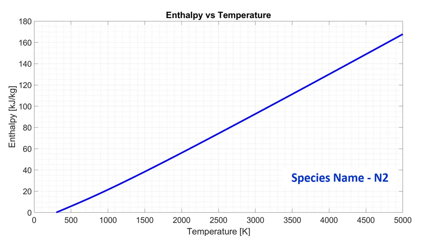
Figure 2b - Enthalpy vs temperature for N2 species

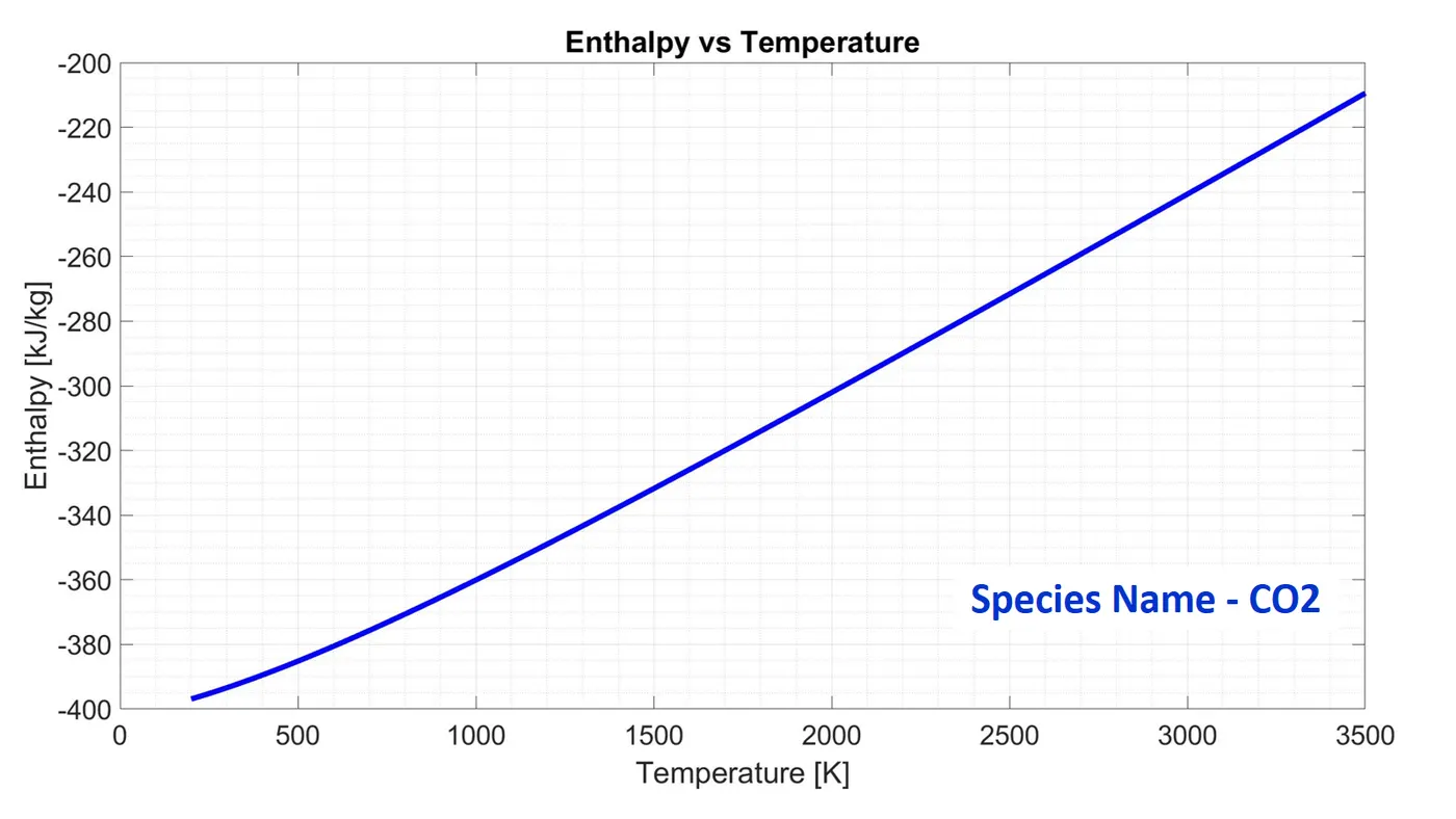
Figure 2c - Enthalpy vs temperature for CO2 species

Figure 2 presents the variation of specific enthalpy (kJ/kg) with temperature. For the three reported species, the trend is almost linear for the high temperature segment (i.e. > 1000 K) but exhibits a slight quadratic behavior for the low temperature range. This can also be approximated as a linear curve fit to an extent. The negative values of enthalpy signify that the chemical reaction is exothermic, i.e. heat is released to the surroundings.

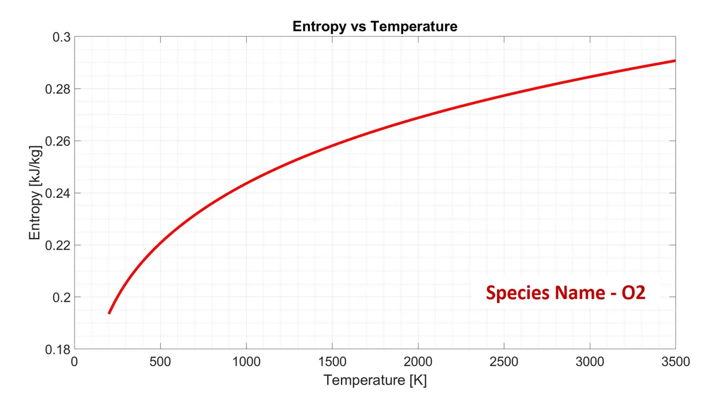
Figure 3a - Entropy vs temperature for O2 species

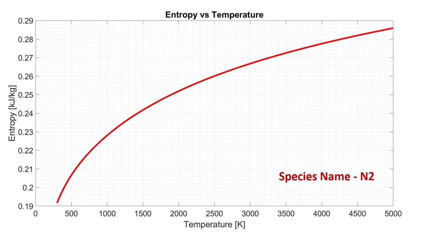
Figure 3b - Entropy vs temperature for N2 species

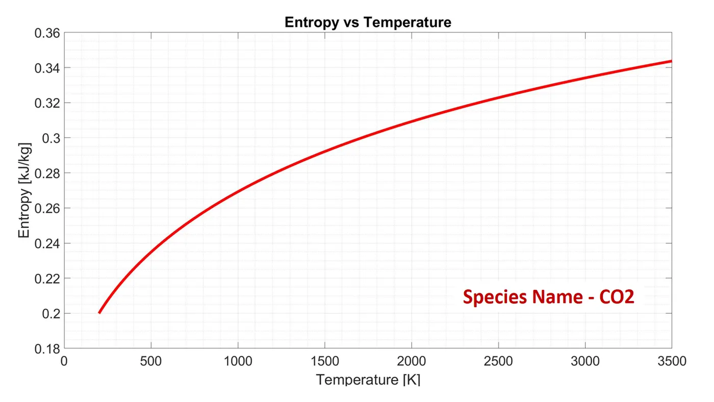
Figure 3c - Entropy vs temperature for CO2 species

Figure 3 shows the specific entropy (kJ/kg) plot for the three species. The trends are similar between the species with some change in the scalar magnitude. The curve exhibits a semi-parabolic behavior over the entire temperature range. The highest value of specific entropy is approximately 0.34 kJ/kg.

Some of the species plots were compared with the published literature in [1] to check if the trends match and they were found to be similar.

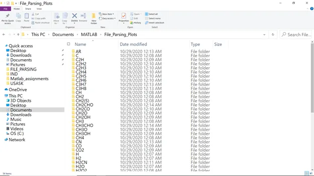
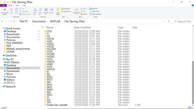
Figure 4 - Screenshots of species folder

Screenshots of saved folders:

The screenshots of the folder where the species directories are saved is shown in Figure 4. A total of 53 species directories are saved with the corresponding `C_p` , h and s plots.

Conclusions:

In this project, the procedure of file parsing was well understood. In addition, using if statements and for loops as needed to optimize the code was a good learning experience. This knowledge can be used to parse any data file and extract relevant information as needed. As a future work, the calculated molecular weights can be written out to a text file for reference and comparison. Any chemical compound can be tracked and studied. The file parsing code has to be tailored to suit the input data file.

References:

1. Matlab Documentation, The MathWorks Inc., 2020
2. Periodic Table of Elements, Sigmaaldrich, 2020

   https://www.sigmaaldrich.com/technical-documents/articles/biology/periodic-table- of-elements-names.html

3. National Institute of Science and Technology: Chemistry Webbook, SRD 69, 2018