Final Project: Electric Rickshaw modelling
Aim:
To create a MATLAB model of an electric rickshaw that uses a battery and a DC motor and observe the output.
Theory:
An EV is a shortened acronym for an electric vehicle. EVs are vehicles that are either partially or fully powered on electric power. Electric vehicles have low running costs as they have fewer moving parts for maintenance and also very environmentally friendly as they use little or no fossil fuels (petrol or diesel). While some EVs used lead-acid or nickel-metal hydride batteries, the standard for modern battery electric vehicles is now considered to be lithium-ion batteries as they have greater longevity and are excellent at retaining energy.
The different types of EV are
- EVs (also known as plug-in electric vehicles) derive all or part of their power from electricity supplied by the electric grid. They include AEVs and PHEVs.
- AEVs (all-electric vehicles) are powered by one or more electric motors. They receive electricity by plugging it into the grid and store it in batteries. They consume no petroleum-based fuel and produce no tailpipe emissions. AEVs include Battery Electric Vehicles (BEVs) and Fuel Cell electric vehicles.
- PHEVs (plug-in hybrid electric vehicles) use batteries to power an electric motor, plug into the electric grid to charge, and use a petroleum-based or alternative fuel to power the internal combustion engine. Some types of PHEVs are also called extended-range electric vehicles (EREVs).
Block diagram:
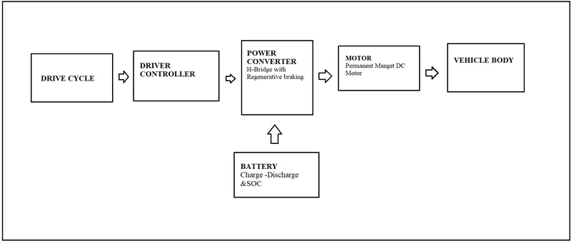
Model:
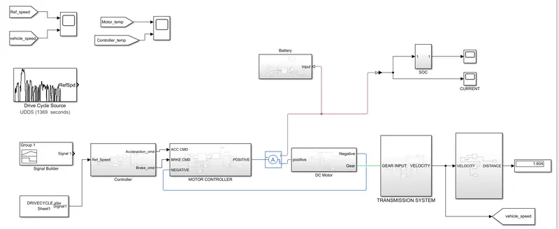
Explanation:
The design of an electric vehicle using a battery and DC Motor consists of 3 subsystems. They are
- Transmission system
- Motor Controller
- SOC Calculation
Transmission System:
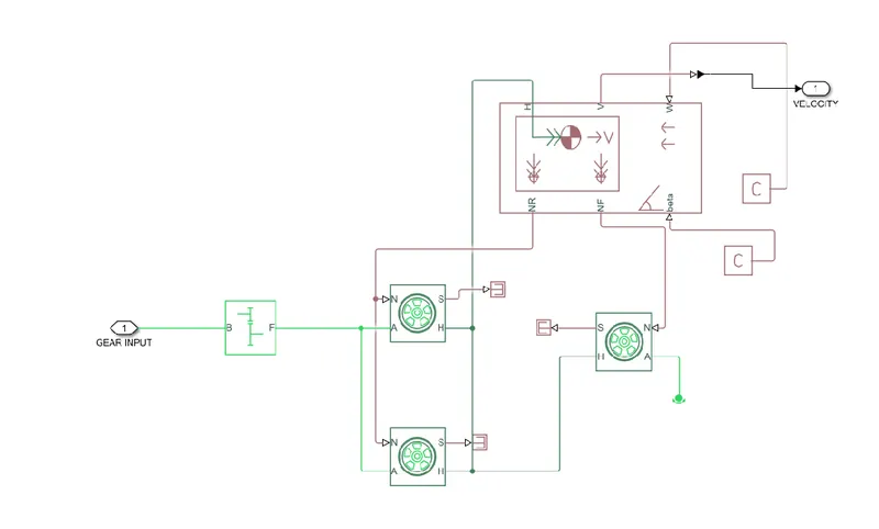
The transmission system consists of the vehicle body, simple gear and Tire(Magic Formula)
Vehicle Body:
The Vehicle body represents a two-axle vehicle body in longitudinal motion. The block accounts for body mass, aerodynamic drag, road incline, and weight distribution between axles due to acceleration and road profile. The vehicle can have the same or a different number of wheels on each axle. Optionally include pitch and suspension dynamics or additional variable mass and inertia. The vehicle does not move vertically relative to the ground.
Connection H is the mechanical translational conserving port associated with the horizontal motion of the vehicle body. The resulting traction motion developed by tires should be connected to this port. Connections V, NF, and NR are physical signal output ports for vehicle velocity and front and rear normal wheel forces, respectively. Wheel forces are considered positive if acting downwards. Connections W and beta are physical signal input ports corresponding to headwind speed and road inclination angle, respectively.
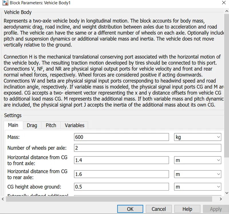
The mass of the vehicle body is kept as 600 kg and parameters are left as default values.
Simple Gear:
The Simple gear represents a fixed-ratio gear or gearbox. No inertia or compliance is modeled in this block. The gear meshing and viscous bearing losses included if necessary. The connections B (base) and F (follower) are mechanical rotational conserving ports.
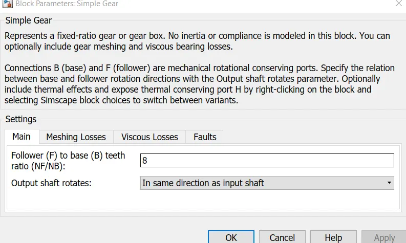
The gear ratio is kept as 8 and the output shaft rotates in the same direction as the input shaft. The friction model is designed as constant efficiency and other values kept default.
Tire(Magic Forumla):
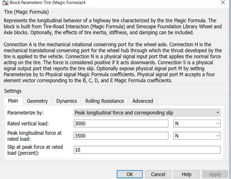
The Tire represents the longitudinal behavior of a highway tire characterized by the tire Magic Formula. The block is built from Tire-Road Interaction (Magic Formula) and Simscape Foundation Library Wheel and Axle blocks. Optionally, the effects of tire inertia, stiffness, and damping can be included.
Explanation of Transmission Subsystem:
Transmission is an important aspect of the vehicle which is used to supply the propulsion power from the motor to wheels. The Tire, simple gear, the vehicle body is used to create the model. Four tire blocks are used which acts on rear wheels and front wheels. During simulation default parameters of the tire are used. Port A represent axle so rear wheels A ports are connected with each other signifies same axles. Similarly, the front wheels are connected. The vehicle body is used which represents the vehicle dynamics where the various parameters can be changed according to the requirement. The NR and NF port of the vehicle body represents the normal force in rear wheels and front wheels, So N port are connected with NR and NF respectively. The Port H represents the horizontal motion of the body and connected to the Port H of all tires. The port V in the vehicle body represents the velocity output from the vehicle. The Port S of all tires can be ignored used they are connected with PS terminator.The power from the motor has to be transmitted to the wheels with help of simple gear blocks. The block is connected to the rear wheel axle since the model considers as rear-wheel drive.Finally the subsystem is modelled where the input of the system is the power given to the simple gear box and output is the velocity of the vehicle.
Motor Controller:
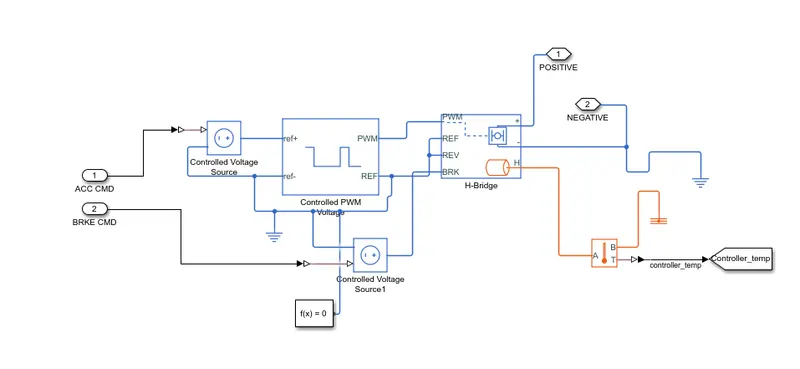
The following blocks are used in the Motor controller System:
- H-bridge
- Controlled Voltage Source
- Controlled PWM Voltage
- Solver Configuration
H-Bridge:
The H-Bridge block represents an H-bridge motor driver. The block has the following two Simulation mode options:
-
PWM — The H-Bridge block output is a controlled voltage that depends on the input signal at the PWM port. If the input signal has a value greater than the Enable threshold voltage parameter value, the H-Bridge block output is on and has a value equal to the value of the Output voltage amplitude parameter. If it has a value less than the Enable threshold voltage parameter value, the block maintains the load circuit using one of the following three Freewheeling mode options:
-
via one semiconductor switch and one freewheeling diode
-
via two freewheeling diodes
-
via two semiconductor switches and one freewheeling diode
-
The first and third options are sometimes referred to as a synchronous operation.
-
-
The signal at the REV port determines the polarity of the output. If the value of the signal at the REV port is less than the value of the Reverse threshold voltage parameter, the output has positive polarity; otherwise, it has negative polarity.
-
Averaged — This mode has two Load current characteristics options:
-
Smoothed
-
Unsmoothed or discontinuous.
-
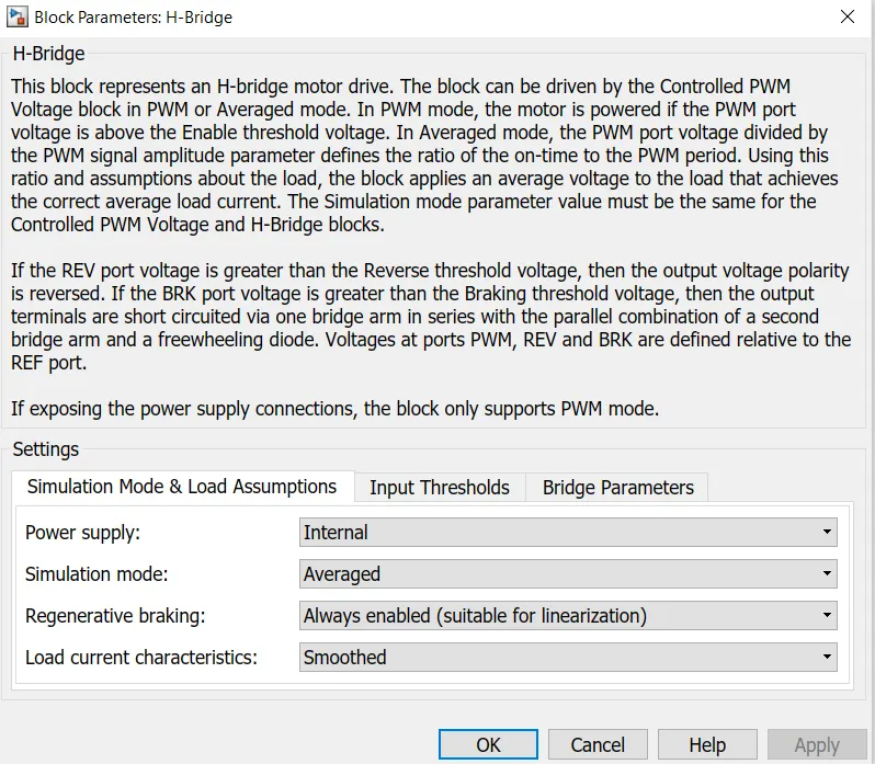
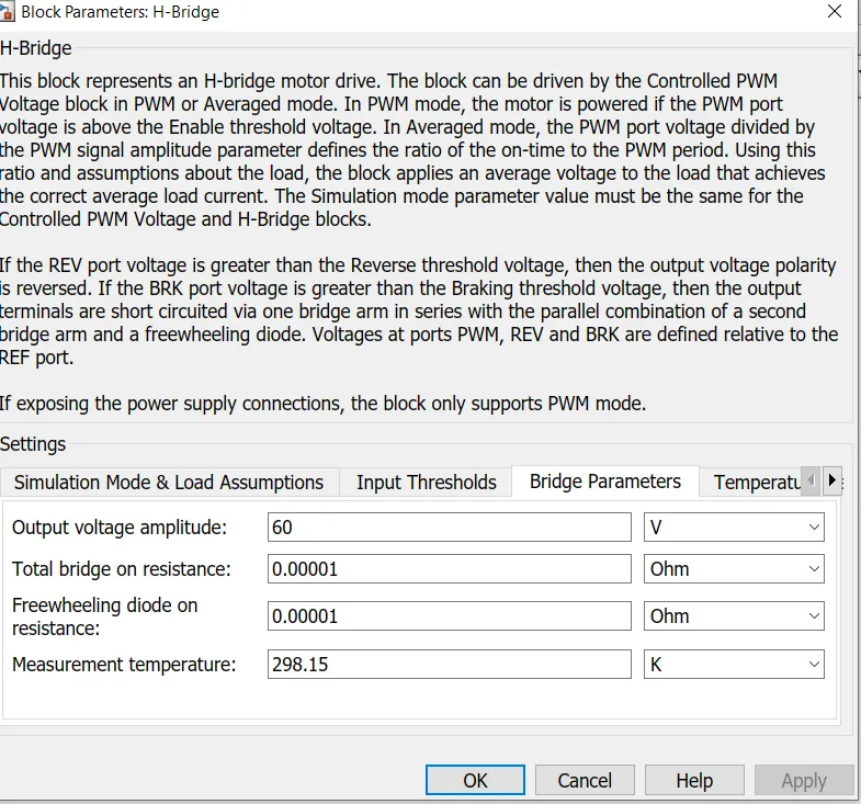
The Simulation mode is set as averaged and load current characteristics are smoothed and the output voltage is 300 V.In Averaged mode, the PWM port voltage divided by the PWM signal amplitude parameter defines the ratio of the on-time to the PWM period.
Controlled PWM Voltage:
This block creates a Pulse-Width Modulated (PWM) voltage across the PWM and REF ports. The output voltage is zero when the pulse is low and is equal to the Output voltage amplitude parameter when high. The duty cycle is set by the input value.
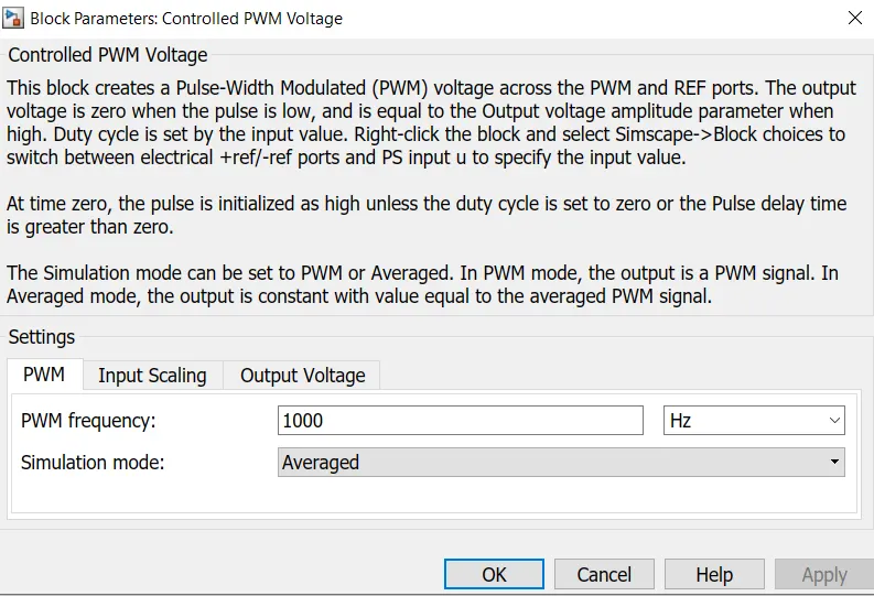
The PWM frequency is set to 600 Hz and the output voltage of the block is 300V.
Controlled Voltage Source:
The block represents an ideal voltage source that is powerful enough to maintain the specified voltage at its output regardless of the current passing through it. The output voltage is V = Vs, where Vs is the numerical value presented at the physical signal port.
Explanation of Motor Controller:
The motor controller subsystem contains mainly H-bridge and Controlled PWM Source block. In H-bridge block parameters averaged mode is chosen since the simulation time is faster than PWM mode. The output voltage amplitude of the H-bridge as DC motor supply voltage. In the H-Bridge the PWM signal port is connected To the PWM output port of the Controlled PWM source and the ref of the Controlled PWM source is connected to the ref,rev,brk of the H_bridge. This block will apply [ulses and based on these pulses from the fixed battery voltage variable voltage will be available to the motor and the motor torque and motor speed are changed.Finally, the subsystem is created with the following blocks and the subsystem will control the power supply of the DC Motor.
SOC Calculation:
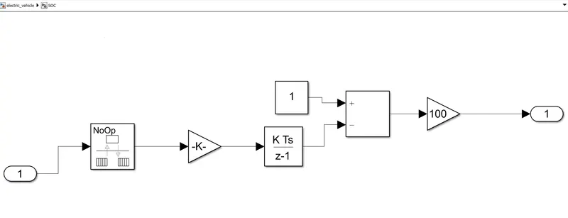
The following Block is used for the SOC Calculation System:
- Rate Transition
- Gain
- Subtract
- Discrete-Time Integrator
Rate Transition:
The Rate Transition block transfers data from the output of a block operating at one rate to the input of a block operating at a different rate.
Gain:
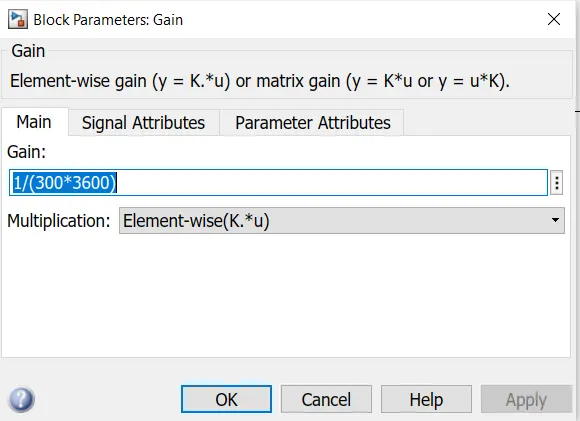
The Gain block multiplies the input by a constant value (gain). The input and the gain can each be a scalar, vector, or matrix.
Discrete-Time Integrator:
The Discrete-Time Integrator block in place of the Integrator block to create a purely discrete model. With the Discrete-Time Integrator block,
-
Define initial conditions on the block dialog box or as input to the block
-
Define an input gain (K) value
-
Output the block state
-
Define upper and lower limits on the integral
-
Reset the state with an additional reset input
Explanation of SOC Calculation:
To measure the state of charge of the battery was created using the various blocks such as Rate Transition, gain and sum blocks. The Current is fed into the Rate transition block and the output of the block is connected to the gain block. Gain block divides the current signal with the voltage rating of the battery multiplied by 3600 seconds in hour.The constant block is used to represent the initial state of charge when performing the simulation and assuming the battery voltage is full the Constant block can be altered with the value representing 100% charge. The signal from the Discrete-time integrator will subtract from the constant block to represent 100% charge. The output of the sum block is fed into the gain block help to convert the output of the sum block in percentage.
Simulink model of Electric Vehicle:
The following blocks are used in the model of Electric Vehicle are
- Drive Cycle
- Controller.
- Battery
- DC Motor
Drive Cycle:
The Block generates a standard or user-specified longitudinal drive cycle. The block output is the vehicle's longitudinal speed.
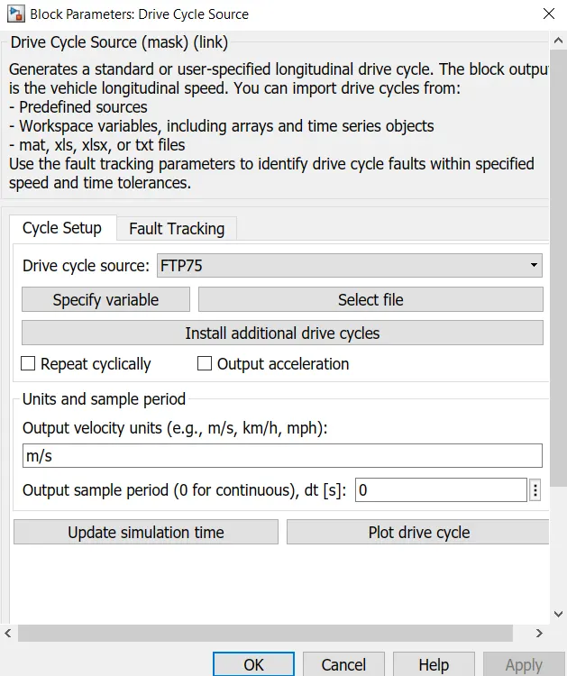
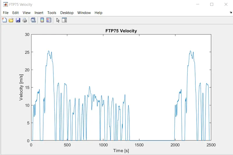
The FTP75 drive cycle is chosen and the drive cycle is plotted in the below figure
Controller:
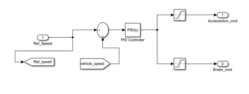
The PID Controller is used to tune the model whereas the input of the block is typically an error signal, which is the difference between a reference signal and the system output. Depending upon the input signal, the acceleration command and brake command are fed into the Motor controller.
DC Motor:
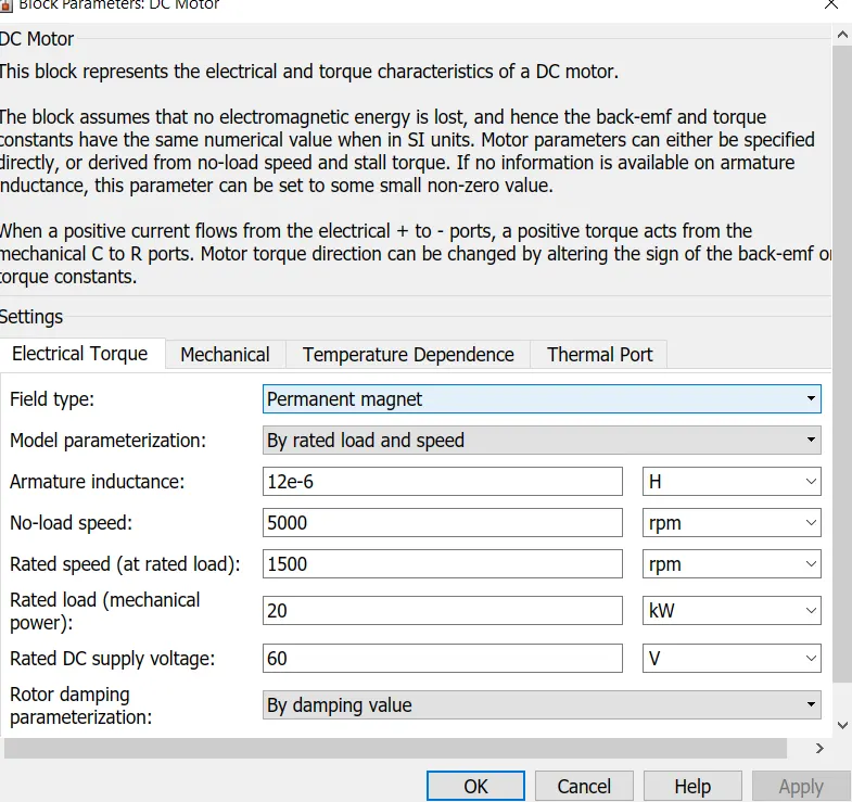
This block represents the electrical and torque characteristics of a DC motor. The block assumes that no electromagnetic energy is lost, and hence the back-emf and torque constants have the same numerical value when in SI units. Motor parameters can either be specified directly or derived from the no-load speed and stall torque. If no information is available on armature inductance, this parameter can be set to some small non-zero value.
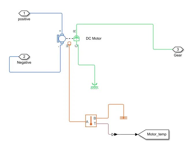
There is two part of DC Motor one is the electrical part and the other one is the mechanical part. The electrical part of the motor is connected to the positive and negative of the H-bridge in the motor controller system. The mechanical part of the DC motor R is connected to the simple gear of the Transmission system and the C part is connected to the Mechanical Rotational Reference.
Distance Calculation:
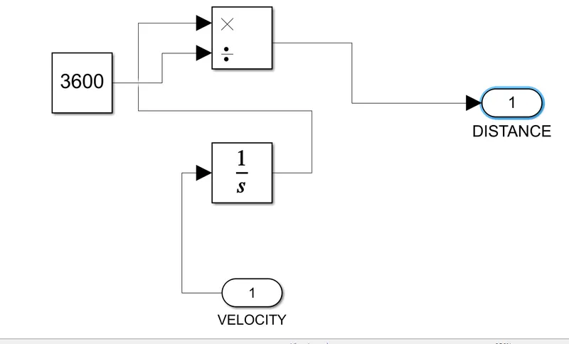
The velocity from the transmission block is fed into the integrator block and divide by 3600 in order to convert the integrated speed which is kmph by 3600 to get the distance traveled by the vehicle.
Explanation of the model:
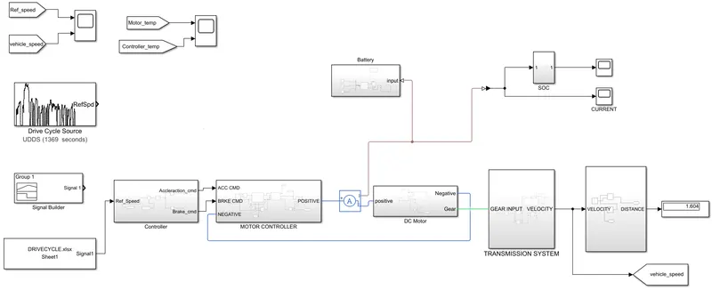
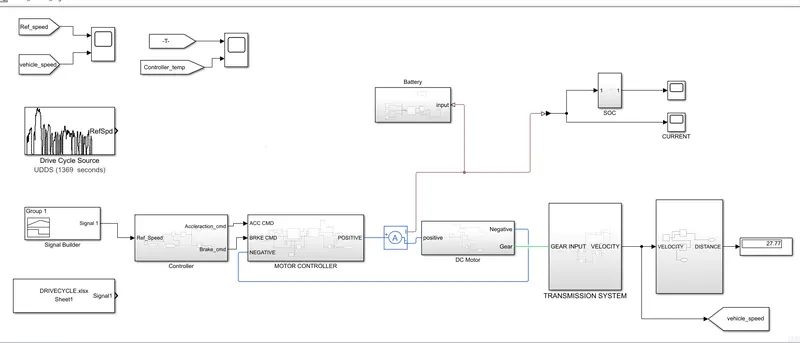
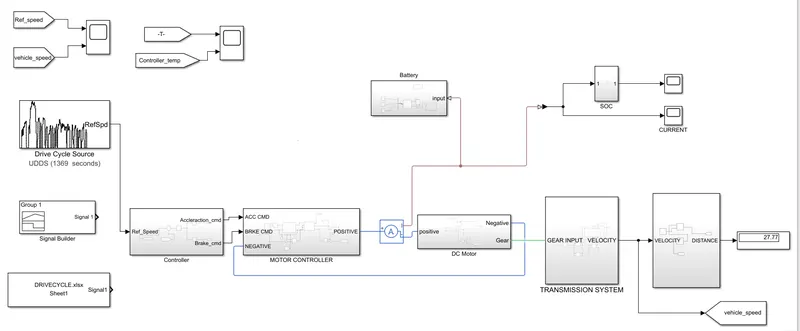
The Drive cycle block is connected to the Controller and vehicle speed is fed back to the controller. Depending upon the vehicle speed acceleration command and deceleration command connected to the controlled PWM source and H-bridge via controlled voltage source in the motor controller system. The motor has 4 parts which + and - are electrical one connected with the H-bridge and the other is mechanical part C and R where mechanical reference and simple gear is connected respectively. In order to measure the speed of the vehicle, the scope is connected to the drive cycle and output velocity from the Transmission block. The distance traveled by the vehicle is calculated using the Distance subsystem. Finally, the EV rickshaw model is completed and once the simulation is run we get the results.
Case Study 1:Drive Cycle - Fed via Excel sheet.
Model:
Result:
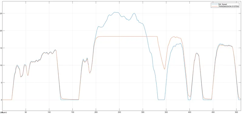
The blue line represents the reference speed and yellow represents the actual velocity of the electric rickshaw. The fine-tuning helps the model follow the exact reference speed. From the above figure, reference speed cant is achievable due to internal circuit constraints of the vehicle.
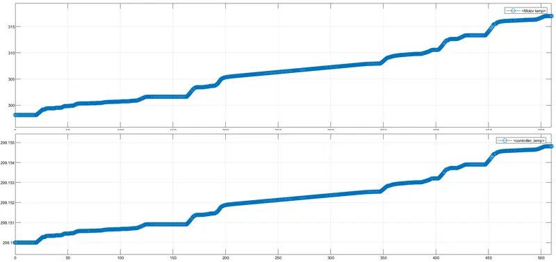
From the above figure, during the acceleration the temperature of the motor and controller rises and during constant speed temperature slightly increases and during the time of deceleration the rises due to the effect of braking.
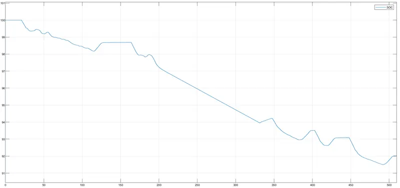
peaks occur during the regenerative braking condition. In this drive cycle, the battery left is 92% and 8% of the charge is depleted by the battery for the completion of the drive cycle.
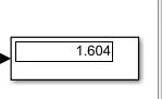
The distance covered by the rickshaw at the end is 1.604 km.
Case Study 2:Drive cycle constant velocity of 45kmph for 100 km.
The cycle has a constant speed of 45kmph which is 12.5m/s for 8000 seconds. The 8000 seconds is calculated via using Speed-Distance-Time Formula.
Model:
Result:
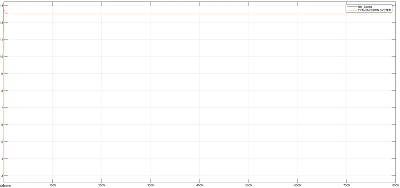
The constant speed is maintained by the vehicle as per reference speed, the initial rise in actual speed due to sudden rise of speed from 0 to 12.5m/s.
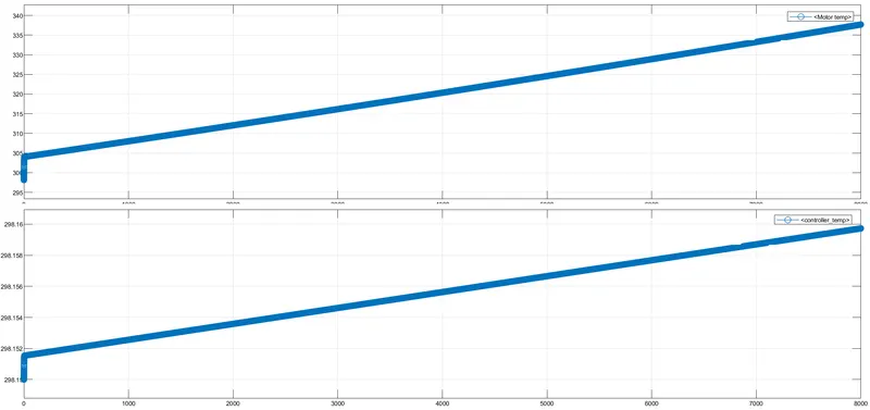
The speed is maintained constant, the temperature of the Motor and controller rise linearly. The 340 degK for the motor and 298.16 degK for the converter temperature.
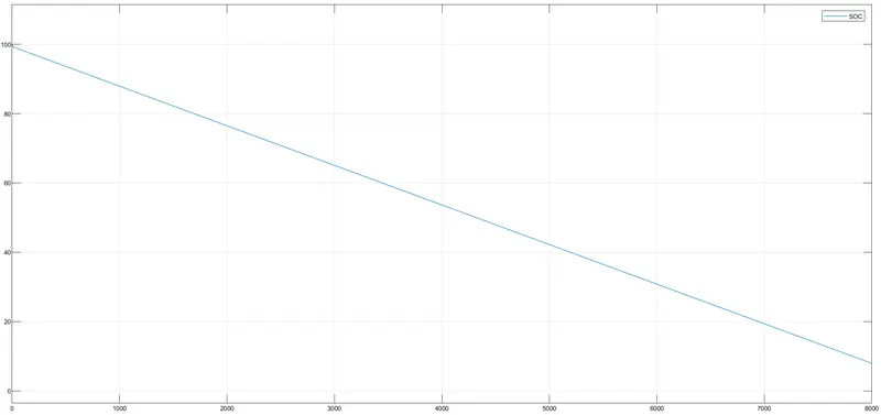
The SOC of the battery will decrease linearly from 100%, which is around 8% charge depletion from the battery.
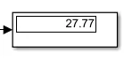
The distance covered by the rickshaw at the end is 27.77 km.
Case Study 3:Drive Cycle Source - UDDS:
Model:
Result:
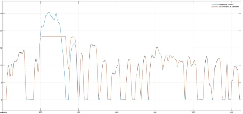
The blue line represents the reference speed and yellow represents the actual velocity of the electric rickshaw. The fine-tuning helps the model follow the exact reference speed. From the above figure, reference speed cant is achievable due to internal circuit constraints of the vehicle.
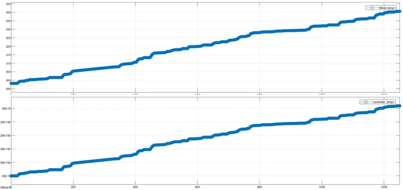
From the above figure, during the acceleration the temperature of the motor and controller rises and during constant speed temperature slightly increases and during the time of deceleration the rises due to the effect of braking.The otor temperatre reaces nearly 345degK and controller temperature is 298.16 degK.
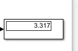
The distance covered by the rickshaw at the end is 3.317 km.
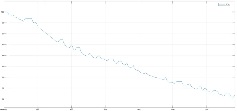
The SOC of the battery will decrease from 100%, which is around 82% charge depletion from the battery.
Conclusion:
The model of the Electric rickshaw has been created and implemented by various drive cycle and explained with a detail analysis.