Final Project: Electric Rickshaw modelling
AIM:-
To build MATLAB model of electric rickshaw (Three wheel passenger vehicle).
OBJECTIVE:
Create a detailed MATLAB model of an electric rickshaw (three wheel passenger vehicle) as per details below:
- Rear wheels driven by PM brushed type motor.
- Assume efficiency points of motor controller and motor.
- Make an excel sheet of all input and assumed data.
BLOCK DIAGRAM:-
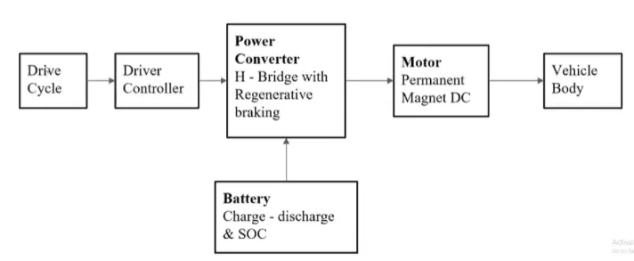
To build Electric rickshaw model there are some main blocks:-
- Drive Cycle:- It is a input to the model.
- Driver Controller :- The block contain controller calculation for acceleration and decceleration values of vehicle.
- Power Converter :- This block contain power converter unit with regenerative braking. DC-DC power converter is to be used here.
- Battery :- The battery block is distributed in 2 blocks one for battery storage discharge unit and another one is for battery state of charge mesuring (SOC).
- Motor:- In this Block DC motor is to be used.
- Vehicle Body :- Block contain Vehicle body like wheel alligment like wise.
MATLAB-SIMULINK MODEL :-
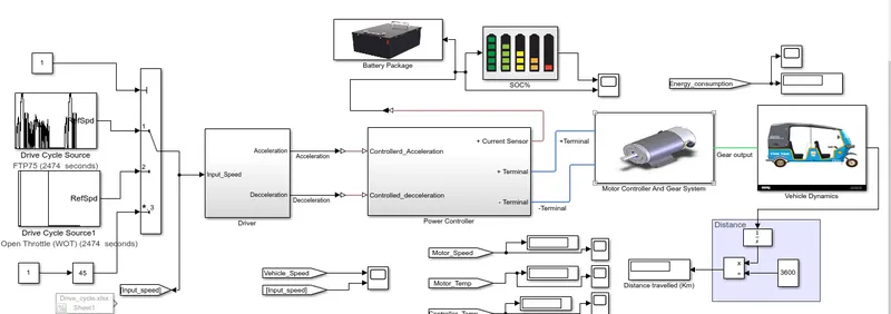
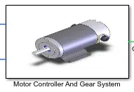
In this model we have used 3 different cycles to check different out puts. Driver control is built by using PID controller. Power Converter Contain H-Bridge DC-DC converter. Motor controller has DC motor with gear system. Vehicle dynamics contain wheel allingment with load distribution. Battery pack and SOC has battery charge discharge calculation and measurment.
1) Vehicle Dynamics :-
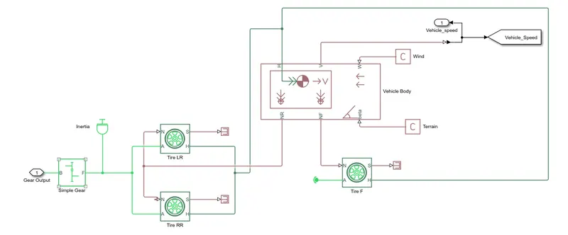
Blocks used:-
- Simple Gear
- Inertia
- Tire
- Vehicle Body
- Simple Gear :-

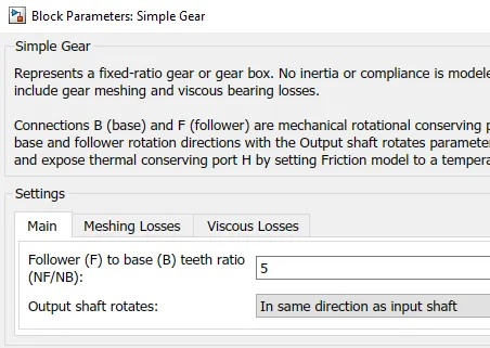
he Simple Gear block represents a gearbox that constrains the connected driveline axes of the base gear, B, and the follower gear, F, to corotate with a fixed ratio that you specify. You choose whether the follower axis rotates in the same or opposite direction as the base axis. If they rotate in the same direction, the angular velocity of the follower, ωF, and the angular velocity of the base, ωB, have the same sign. If they rotate in opposite directions, ωF and ωB have opposite signs.
Settings :-
- Inertia :-
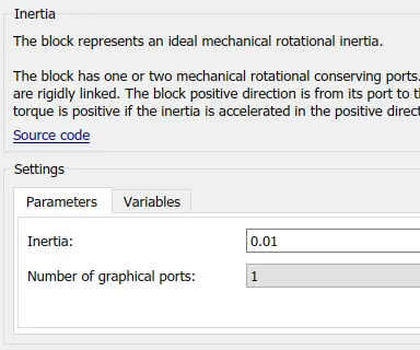
The Inertia block represents an ideal mechanical translational inertia that is described with the following equation:
T=Jdωdt
where:
-
T is inertia torque.
-
J is inertia.
-
ω is angular velocity.
-
t is time.
By default, the block has one mechanical translational conserving port. The block positive direction is from its port to the reference point. This means that the inertia torque is positive if inertia is accelerated in the positive direction.
In some applications, it is customary to display inertia in series with other elements in the block diagram layout. To support this use case, the Number of graphical ports parameter lets you display a second port on the opposite side of the block icon. The two-port variant is purely graphical: the two ports have the same angular velocity, so the block functions exactly the same whether it has one or two ports. The block icon changes depending on the value of the Number of graphical ports parameter.
Settings :-
- Tire :-

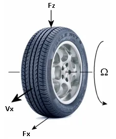
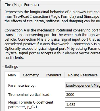
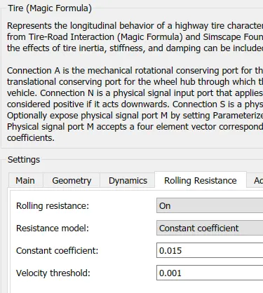
The Tire (Magic Formula) block models the tire as a rigid wheel-tire combination in contact with the road and subject to slip. When torque is applied to the wheel axle, the tire pushes on the ground (while subject to contact friction) and transfers the resulting reaction as a force back on the wheel. This action pushes the wheel forward or backward. If you include the optional tire compliance, the tire also flexibly deforms under load.
Input
N - Normal Force :- Physical signal input port associated with the normal force acting on the tire. The normal force is positive if it acts downward on the tire, pressing it against the pavement.
Output
S - Slip :- Physical signal output port associated with the relative slip between the tire and road.
Conserving
A - Axle :- Mechanical rotational port associated with the axle that the tire sits on.
H - Hub :- Mechanical translational port associated with the wheel hub that transmits the thrust generated by the tire to the remainder of the vehicle.
Settings :-
Rolling Radius :- 0.32 m
Velocity Threshold :- 0.1 m/s
- Vehicle Body:-
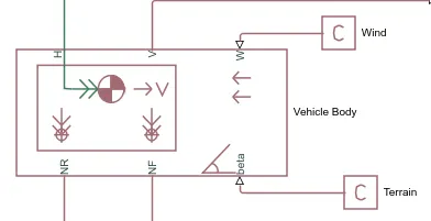
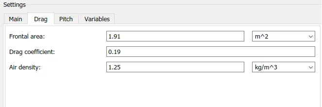
The Vehicle Body block represents a two-axle vehicle body in longitudinal motion. The vehicle can have the same or a different number of wheels on each axle. For example, two wheels on the front axle and one wheel on the rear axle. The vehicle wheels are assumed identical in size. The vehicle can also have a center of gravity (CG) that is at or below the plane of travel.
The block accounts for body mass, aerodynamic drag, road incline, and weight distribution between axles due to acceleration and road profile. Optionally include pitch and suspension dynamics. The vehicle does not move vertically relative to the ground.
The block has an option to include an externally-defined mass and an externally-defined inertia. The mass, inertia, and center of gravity of the vehicle body can vary over the course of simulation in response to system changes.
Ports
Input
W - Headwind speed, m/s :- Physical signal input port for headwind speed.
beta - Road incline angle, rad :-Physical signal input port for road incline angle.
Output
V - Longitudinal Velocity, m/s :- Physical signal output port for vehicle longitudinal velocity.
NF - Front axle normal force, N :-Physical signal output port for normal force on the front axle. Wheel forces are considered positive if acting downwards.
Nr - Rear axle normal speed, N :-Physical signal output port for normal force on the rear axle. Wheel forces are considered positive if acting downwards.
Conserving
H - Horizontal motion :-Conserving port associated with the horizontal motion of the vehicle body. Connect tire traction motion to this port.
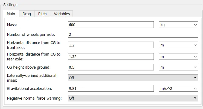
Settings:-
2) Motor Control and Gear System
Blocks Used :-
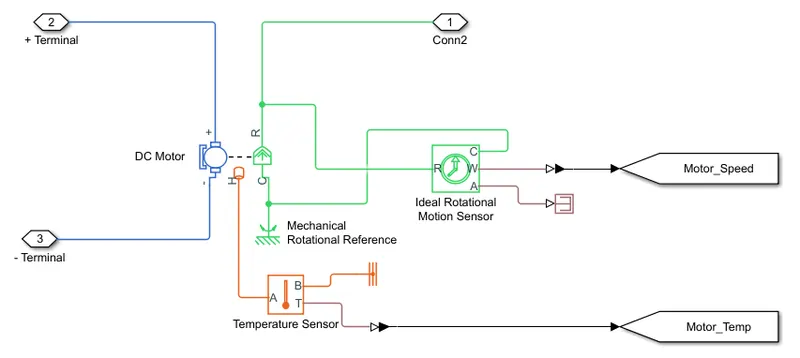
- DC Motor
- Thermal Sensor
- Ideal Rotational Motion Sensor
DC Motor :-
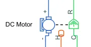
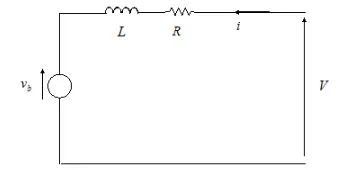
You specify the equivalent circuit parameters for this model when you set the Model parameterization parameter to By equivalent circuit parameters . The resistor R corresponds to the resistance you specify in the Armature resistance parameter. The inductor L corresponds to the inductance you specify in the Armature inductance parameter.
- For the steady-state torque-speed relationship, L has no effect.
- Sum the voltages around the loop and rearrange for i:
i=V−vbR=V−kvωR
- Substitute this value of i into the equation for torque:
TE=ktR(V−kvω)
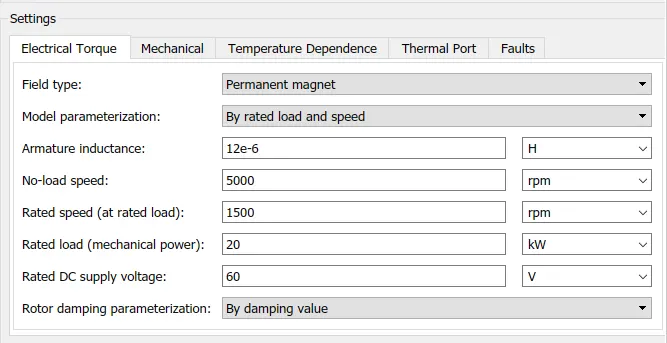
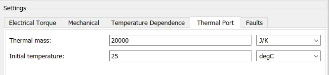
Settings :-
Thermal Sensor :-
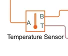
The Temperature Sensor block represents an ideal temperature sensor, that is, a device that determines the temperature differential measured between two points without drawing any heat.
Connections A and B are thermal conserving ports that connect to the two points where temperature is being monitored. Port T is a physical signal port that outputs the temperature differential value.
The block positive direction is from port A to port B. The measured temperature is determined as T = TA – TB.
Ports
The block has the following ports:
- A :- Thermal conserving port associated with the sensor positive probe.
- B :- Thermal conserving port associated with the sensor negative probe.
- T :- Physical signal output port for temperature.
Ideal Rotational Motion Sensor :-
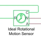
The Ideal Rotational Motion Sensor block represents an ideal mechanical rotational motion sensor, that is, a device that converts an across variable measured between two mechanical rotational nodes into a control signal proportional to angular velocity or angle. The initial angular position can be specify (offset) as a block parameter. Connections R and C are mechanical rotational conserving ports that connect the block to the nodes whose motion is being monitored. Connections W and A are physical signal output ports for velocity and angular displacement, respectively. The block positive direction is from port R to port C. This means that the velocity is measured as ω = ωR – ωC, where ωR, ωC are the absolute angular velocities at ports R and C, respectively.
Ports
Output
W - Angular velocity, rad/s :- Physical signal output port for angular velocity.
A - Angular Displacement :- Physical signal output port for angular displacement.
Conserving
R - Rod :- Mechanical rotational conserving port associated with the sensor positive probe.
C - Case :- Mechanical rotational conserving port associated with the sensor negative (reference) probe.
3) Power Controller
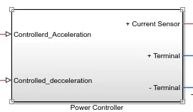
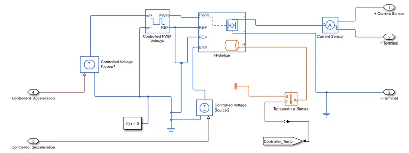
Blocks Used :-
- H-Bridge
- Controlled PWM voltage
- Controlled Voltage Sensor
- Current Sensor
- Temperature Sensor
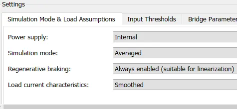
H - Bridge :-
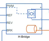
An H-bridge is an electronic circuit that switches the polarity of a voltage applied to a load. These circuits are often used in robotics and other applications to allow DC motors to run forwards or backwards.
Ports
PWM - Pulse with modulation signal :- Electrical conserving port associated with the pulse-width modulated signal. The voltage is defined relative to the REF port.
REF - Reference :- Electrical conserving port associated with the floating zero volt reference.
REV :- Electrical conserving port associated with the voltage that controls when to reverse the polarity of the H-Bridge block output. The voltage is defined relative to the REF port.
BRK :- Electrical conserving port associated with the voltage that controls when to short circuit the H-Bridge block output. The voltage is defined relative to the REF port.
+ ve - Positive load connection port :- Electrical conserving port associated with the positive load connection.
- ve - Negetive load connection port :- Electrical conserving port associated with the negative load connection.
H - Thermal port
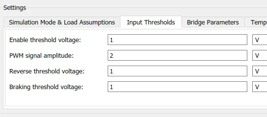
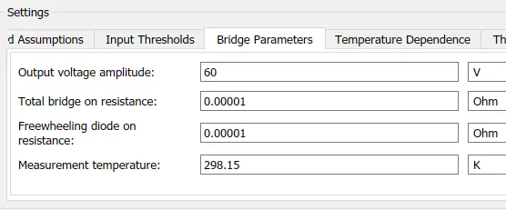
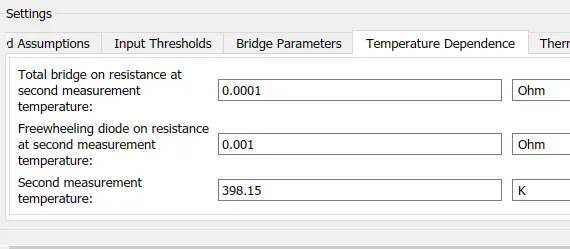
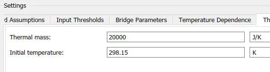
Settings :-
Controlled PWM voltage :-

The Controlled PWM Voltage block represents a pulse-width modulated (PWM) voltage source.
Ports
ref+ - Positive terminal :- Positive electrical reference voltage.Enabled for the Electrical input ports variant of the block.
ref- - Negetive terminal :- Negative electrical reference voltage. Enabled for the Electrical input ports variant of the block.
PWM - Pulse width modulation signal :- Electrical conserving port associated with the pulse-width modulated signal.
REF - Floting Zero volts reference :- Electrical conserving port associated with the floating zero volt reference.
Settings :-
PWM frequency: 1000Hz
Input voltage for 0% duty cycle: 0V
Input voltage for 100% duty cycle: 2V
Output voltage amplitude: 60V
Controlled Voltage Sensor
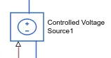
The Controlled Voltage Source block represents an ideal voltage source that is powerful enough to maintain the specified voltage at its output regardless of the current flowing through the source.
The output voltage is V = Vs, where Vs is the numerical value presented at the physical signal port.
Ports
The block has one physical signal input port and two electrical conserving ports associated with its electrical terminals.
Current Sensor

The Controlled Voltage Source block represents an ideal voltage source that is powerful enough to maintain the specified voltage at its output regardless of the current flowing through the source.
The output voltage is V = Vs, where Vs is the numerical value presented at the physical signal port.
Ports
The block has one physical signal input port and two electrical conserving ports associated with its electrical terminals.
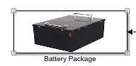
4) Battery pack
Blocks Used :-
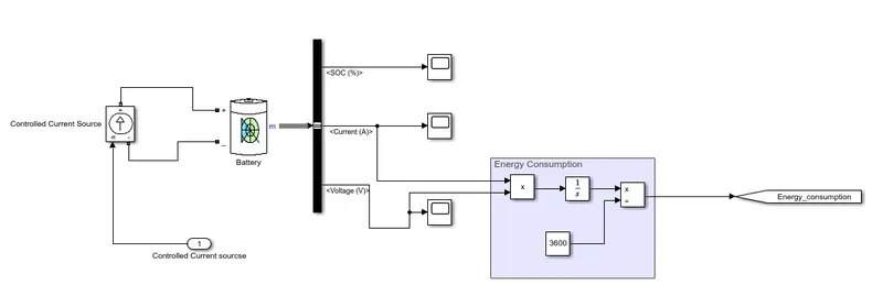
- Battery
- Controlled current source
- Energy Consumption calculations
Battery
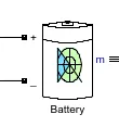
The Battery block implements a generic dynamic model that represents most popular types of rechargeable batteries.
ports
m - Output vector of signals for the battery temperature, state-of-charge, current, voltage, age, maximum capacity, and the ambient temperature.
+ve - Specialized electrical conserving port associated with the battery's positive terminal.
-ve - Specialized electrical conserving port associated with the battery's positive terminal.
Settings :-
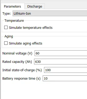
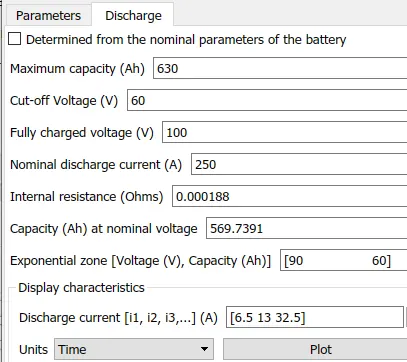
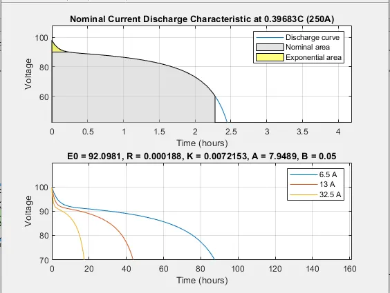
Plot according to settings
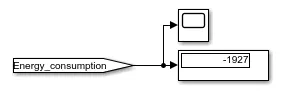
Energy Consumption Calculation
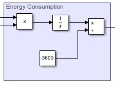
Multiplying the current and voltage output value, calculate Integrated value and 3600 for energy consumption value.
5) SOC
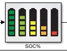
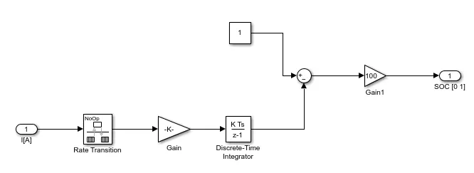
Input I(A) from battery.
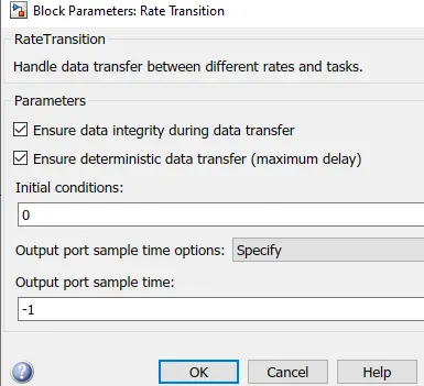
Rate Transition (Settings):-
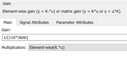
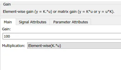
Gain and Gain1:-
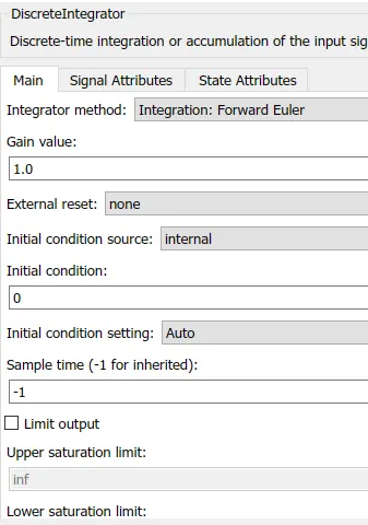
Discrete-Time Integrator :-
6) Driver
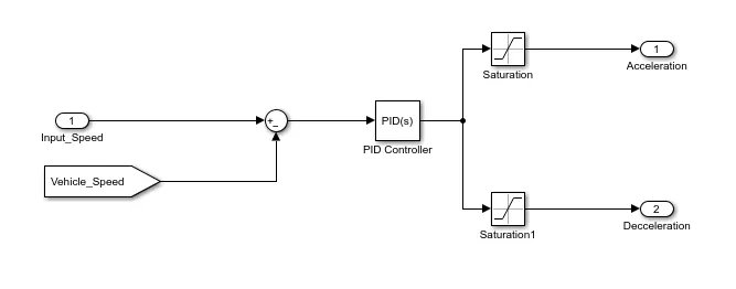
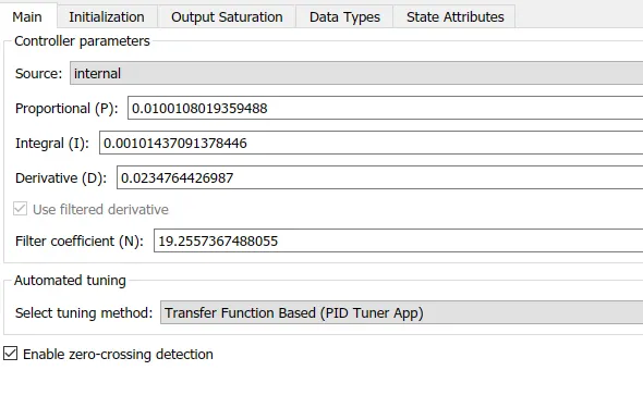
PID Controller
Output according Input to Drive Cycle:-
INPUT 1
FTP75 (2474 sec) :-
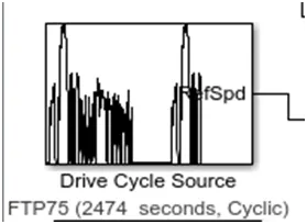
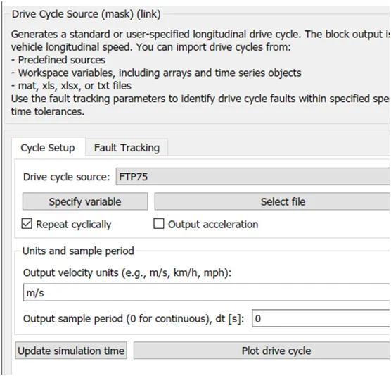
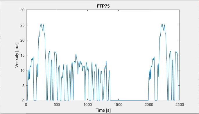
FTP 75 is one of the standard drive cycle which is used for 2474 sec. By keeping the other parameter as it is
OUTPUT 1
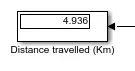
- Distance travelled
- Input and vehicle speed
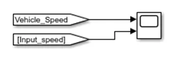
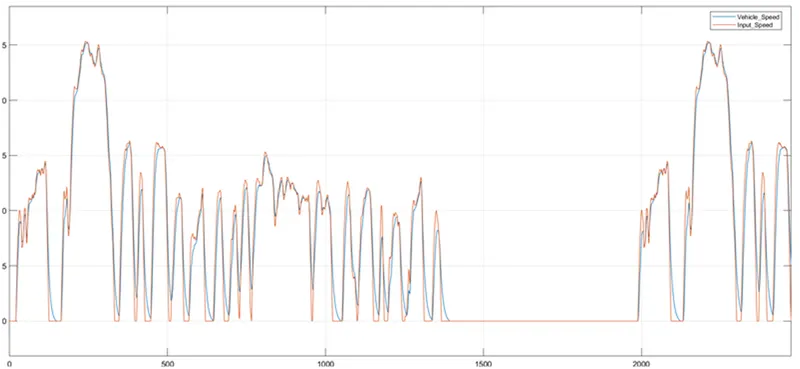
Here blue line shows Vehicle speed which following red line which is Input speed given by drive cycle.
- Motor Speed

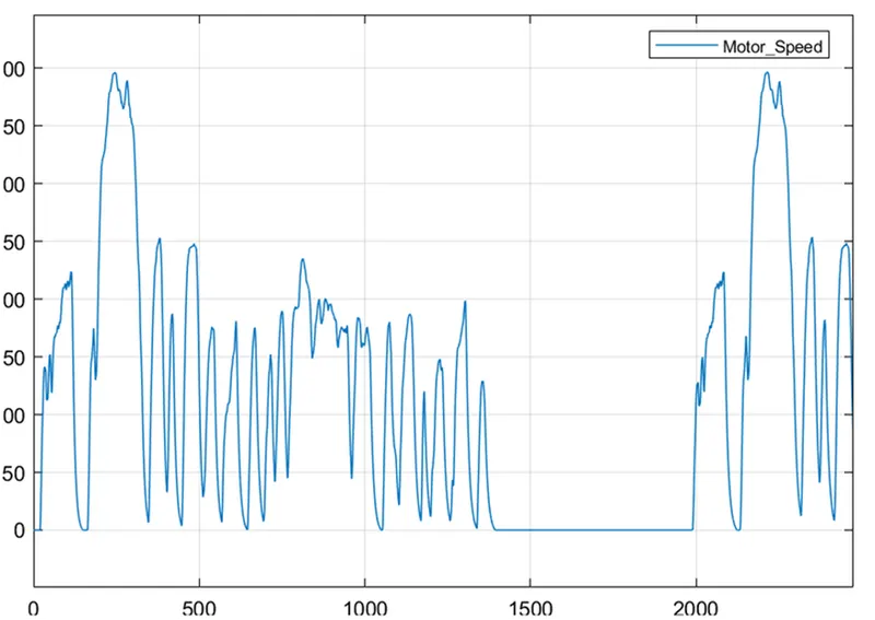
- Output from Battery
SOC%, Current, Voltage
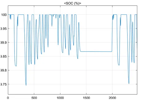
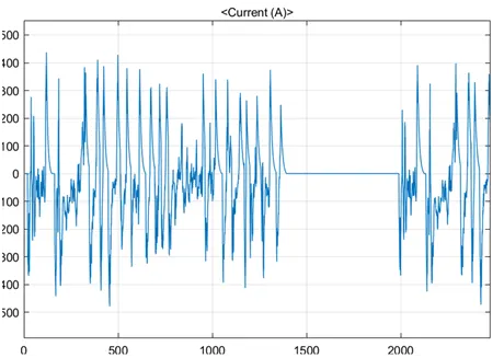
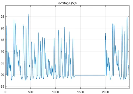
- Output From SOC block
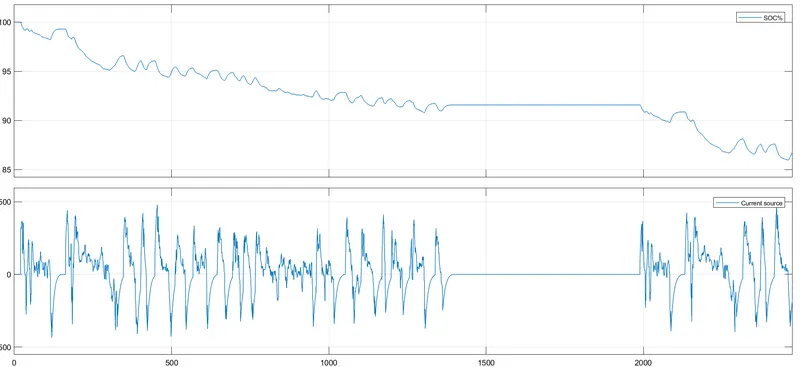
Result 1
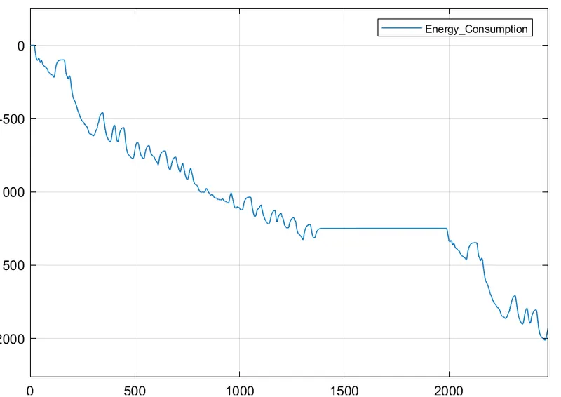
- Energy Consumption
Energy Consumption shows in Negetive value because of use of energy.
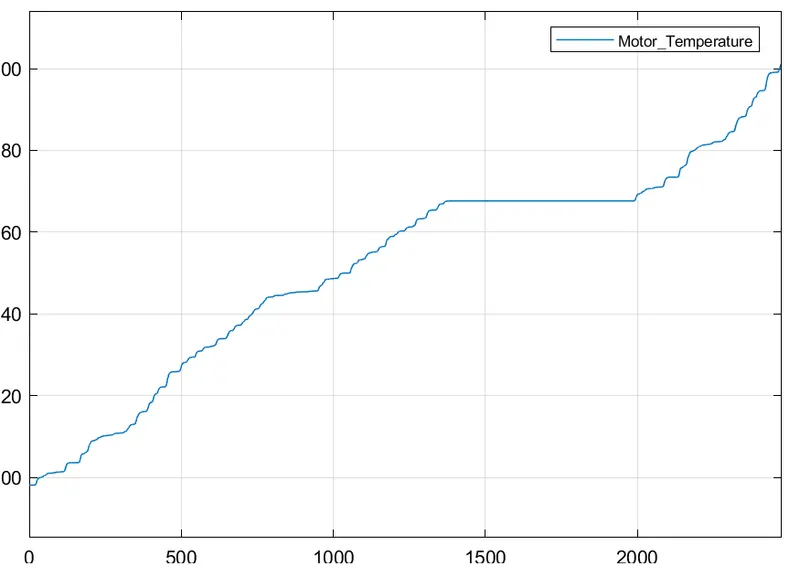
- Motor Temperature

After runing for 4.9 km of FTP75 cycle the motor temperature is 401.2 K at the end of the cycle.
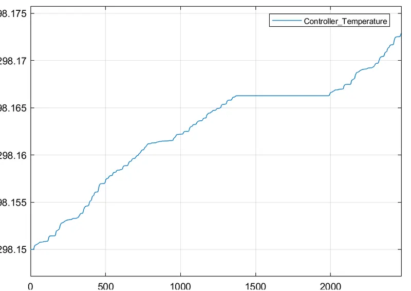
- Controller Temperature

After runing for 4.9 km of FTP75 cycle the controller temperature is 298.2 K at the end of the cycle.
INPUT 2
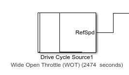
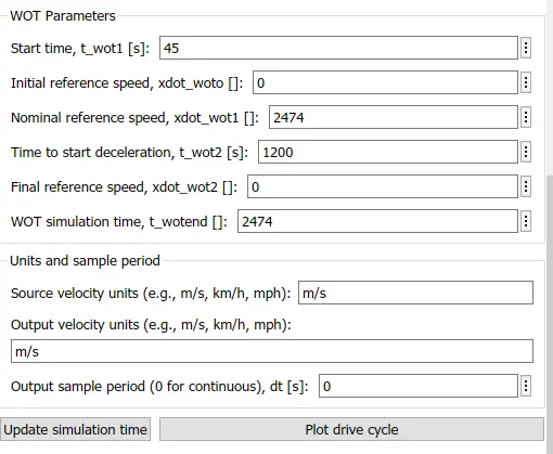
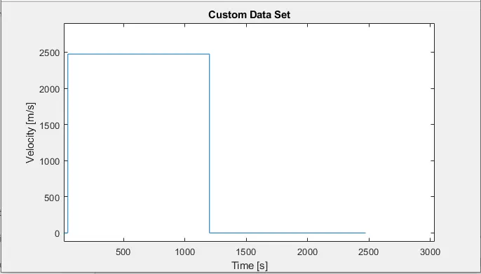
Wide Open Throttle (WOT) (2474 sec)
OUTPUT 2
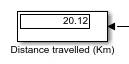
- Distance travelled
- Input and vehicle speed
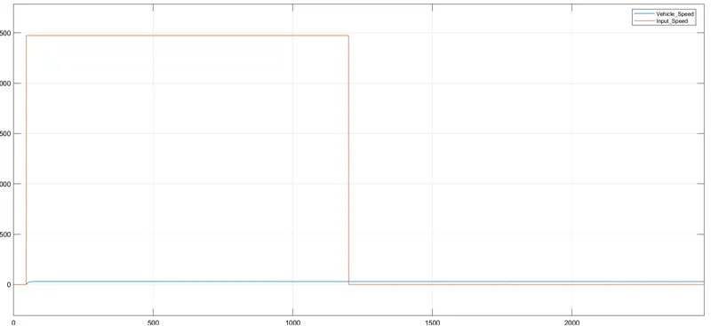
Here blue line shows Vehicle speed which following red line which is Input speed given by drive cycle.
- Motor Speed
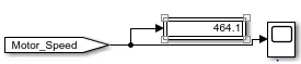
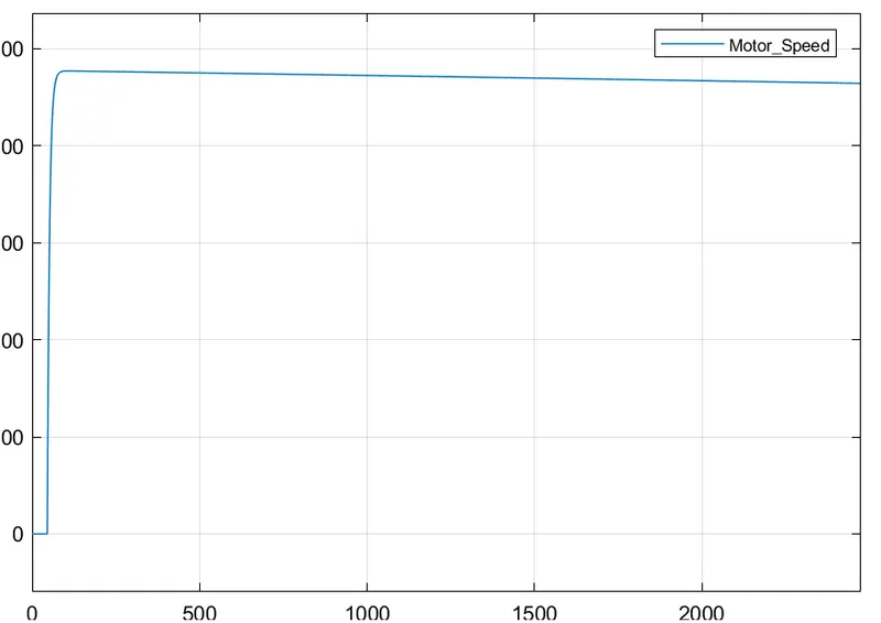
- Output from Battery
SOC%, Current, Voltage
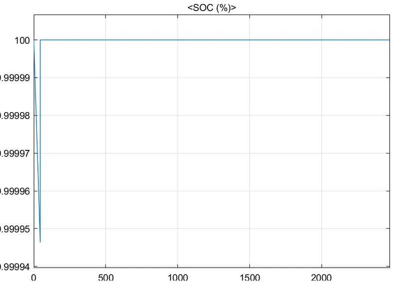
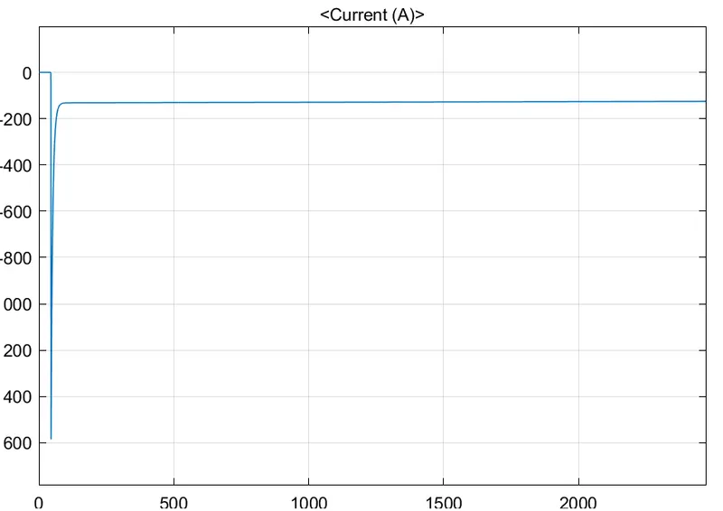
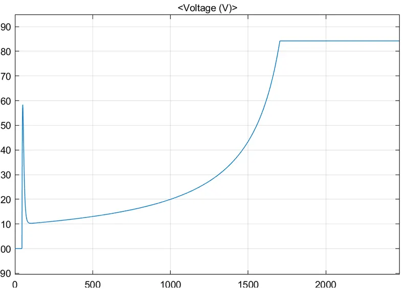
- Output From SOC block
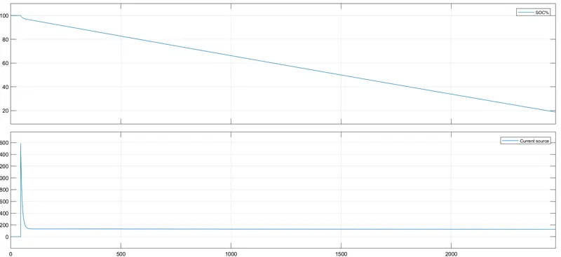
Result 1
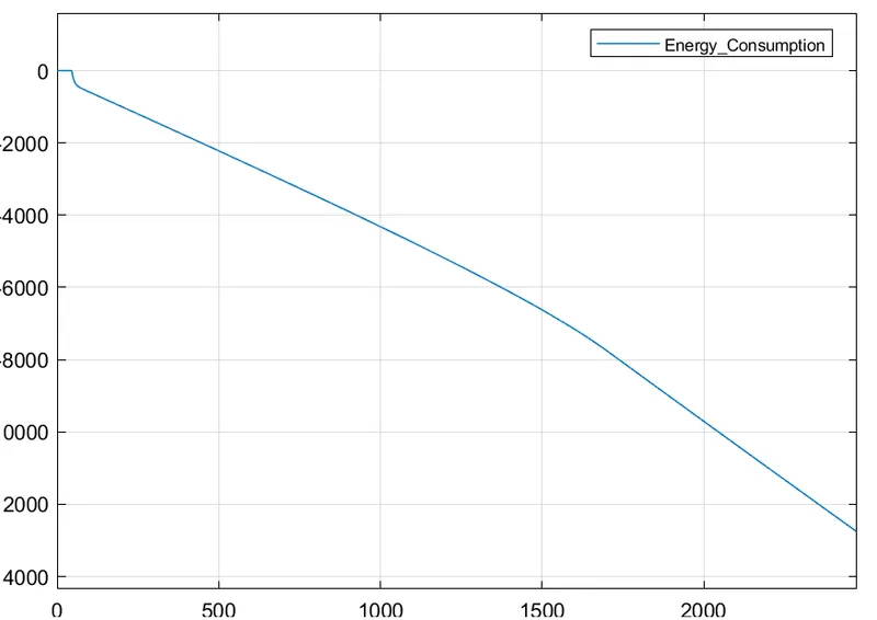
- Energy Consumption
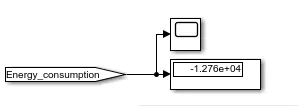
Energy Consumption shows in Negetive value because of use of energy.
- Motor Temperature

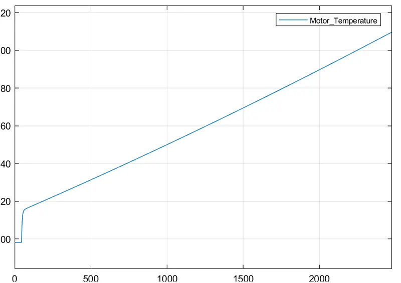
After runing for 20.12 km of WOT cycle the motor temperature is 409.8 K at the end of the cycle.
- Controller Temperature

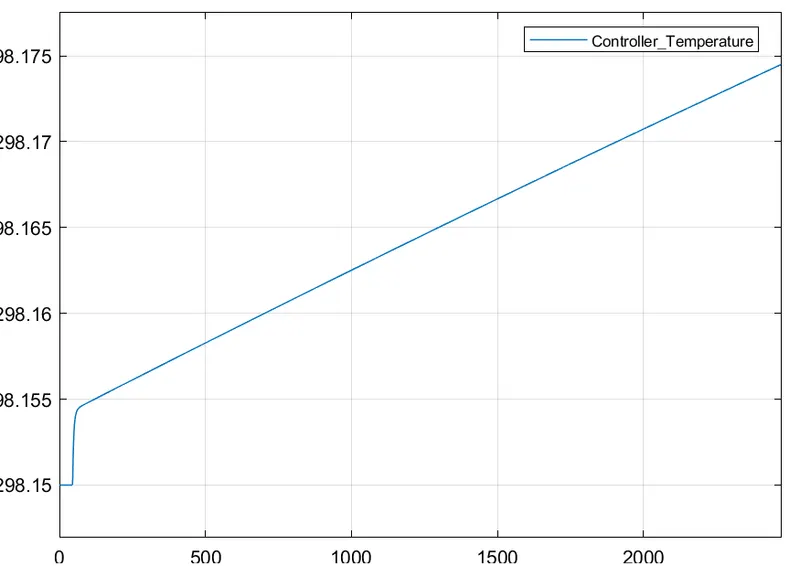
After runing for 20.12 km of WOT cycle the controller temperature is 298.2 K at the end of the cycle.
INPUT 3
Slider Gain Block
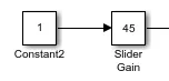
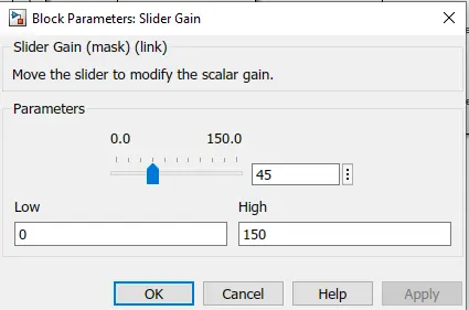
Travelling for 100 km at 45kmph speed need 12879 sec to run the program using Slider gain block. Which is used as drive cycle for rikshaw model.
OUTPUT 3
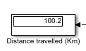
- Distance travelled
- Input and vehicle speed
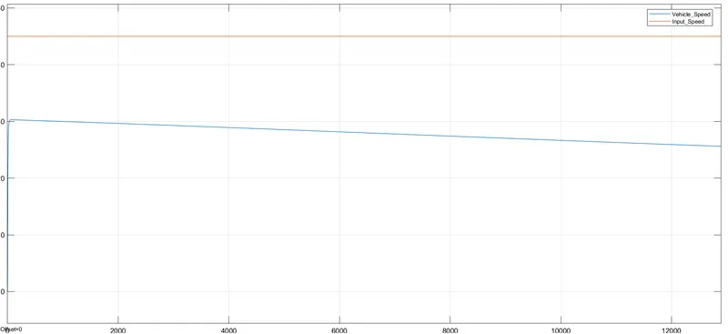
Here blue line shows Vehicle speed which following red line which is Input speed given by drive cycle. the input vehicle speed is constant for 45 kmph.
- Motor Speed

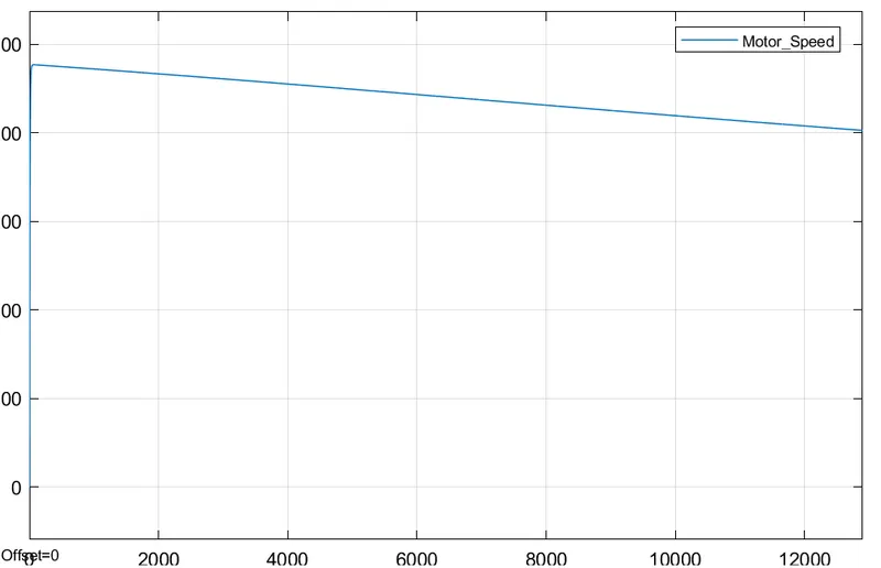
- Output from Battery
SOC%, Current, Voltage
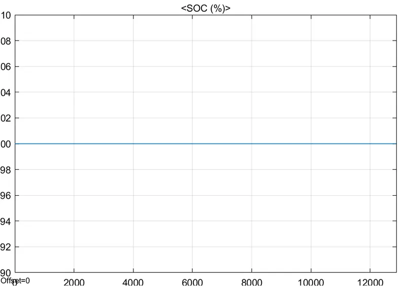
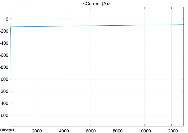
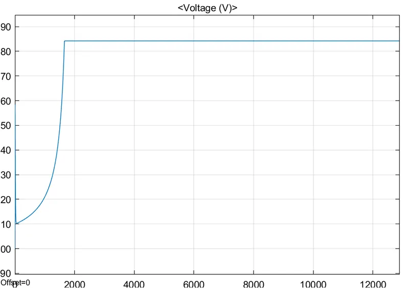
- Output From SOC block
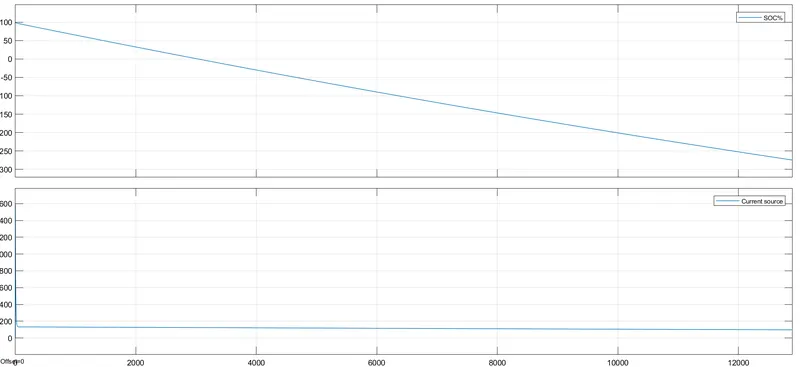
Result 1
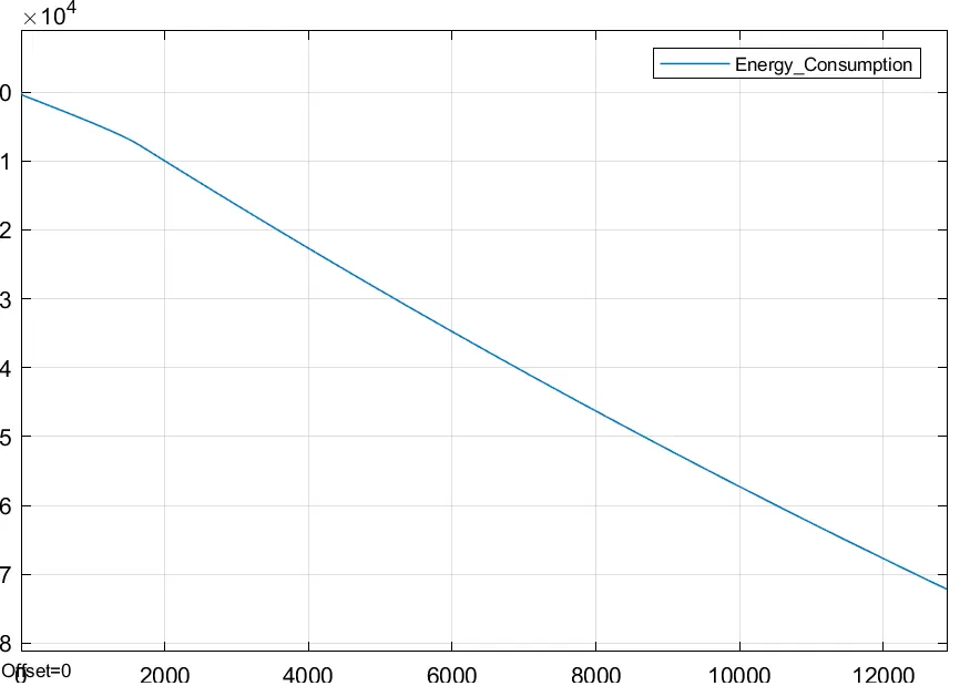
- Energy Consumption
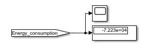
Energy Consumption shows in Negetive value because of use of energy.
- Motor Temperature

After runing for 100 km of slider gain cycle the motor temperature is 1003 K at the end of the cycle.
- Controller Temperature
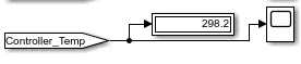
After runing for 100 km of Slider Gain cycle the controller temperature is 298.2 K at the end of the cycle.
Final Result :-
| Type of Drive Cycle | Simulation Time | Distance Travelled | Energy Consumption | Motor Temperature | Controller Temperature |
| FTP75 | 2474 sec | 4.936 km | -1972 N | 401.2 K | 298.2 K |
| WOT | 2474 sec | 20.12 km | -1.276e+04 N | 409.8 K | 298.2 K |
| Slider Gain | 12879 sec | 100.2 km | -7.223e+04 N | 1003 K | 298.2 K |
Conclusion :-
- As we see by applying different drive cycle to rickshaw model for different simulation time there is difference in distance travelled in given time.
- Energy consumption is more in Slider gain drive cycle.
- Also the motor temperature is higher in Slider gain with constant speed of vehicle for 100km.
- Controller temperature is constant for all the cycles.
Attachments:-
- Simulink model of rickshaw.
- Excel file, including all the parameters to be set to run the model.