Final Project: Design of an Electric Vehicle
Aim :
Create a MATLAB model of electric car which uses a battery and a DC motor. Choose suitable blocks from Powertrain block set. Prepare a report about your model including following:
Objectives:
1. System level configurations
2. Model parameters
3. Results
4. Conclusion
THEORY :
An Electric Vehicle (EV) is a vehicle that uses one or more electric motors or traction motors for propulsion. An electric vehicle may be powered through a collector system by electricity from off-vehicle sources, or may be self-contained with a battery, solar panels, fuel cells or an electric generator to convert fuel to electricity. EVs include, but are not limited to, road and rail vehicles, surface and underwater vessels, electric aircraft and electric spacecraft.
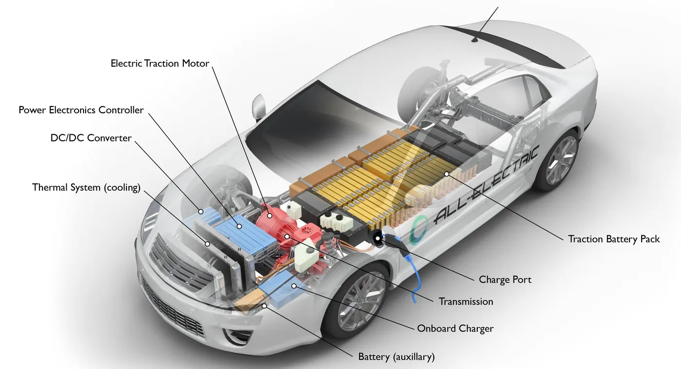
Components of an EV -
- EVs have no need for the fuel engine and gear transmission, the two of the most crucial components for internal combustion vehicles.
- An electric powered car has three primary components - Battery, motor controller, and the electric motor.
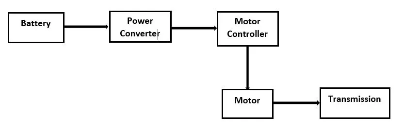
(1) Battery : The battery of an electric car can be charged through the use of ordinary grid electricity at a specialized power station. But aside from the conventional lithium-ion battery technologies, there are also other major battery technologies which can be used for electric cars.
- Lithium-Ion Batteries : This battery technology gives extra performance and range. However, it also carries the highest price tag. Lithium-ion batteries are lighter than Lead acid and Nickel metal. These are also the batteries used in digital cameras and smartphones.
- Lead Acid Batteries : This battery technology is the most popular. It is also the cheapest among the battery technologies. What’s good about it is it’s 97% recyclable.
- Nickel Metal Hydride Batteries : This battery technology provides higher output and better performance but it costs much more than lead-acid batteries.
(2) Motor Controller : The motor controller of an electric car administers its complete operation and the distribution of its power at any given moment. It acts as a floodgate between the motor and batteries. It helps monitor and regulates all key performance indications such as the vehicle’s operator, motor, battery, and accelerator pedal. It has a microprocessor which can limit or redirect current. It is used to either improve the mechanical performance of the car or suit the operator’s driving style. There are also more refined controllers which are capable of greater accuracy and thus, higher efficiency.
(3) Electric Motor : Unlike a gasoline engine with lots of moving parts, a motor only has one moving part. This makes it a very reliable source of motive power. Choosing an electric motor depends on the car’s system voltage. They can be structured to use either AC or DC current. AC motors are less expensive and lighter compared to DC motors. They are also more common and they tend to suffer from less mechanical wear and tear. However, AC technology requires a more refined or sophisticated motor controller.
We will use following parameters for the vehicle body and tires and following condition for the wind and terrain.
Vehicle mass : 1000 kg
Wheels per axle : 2
Frontal area : 3m^2
Drag coefficent : 0.02
Tire ( Magic_Formula )
Rolling radious (r) : 0.3 m
Rolling resistance : 0.015
Now Let's calculate all the requeird data for desiging
1. Forces acting on the vehicle
A] Rolling resistance force
Frr = urr mg
Where, Frr is the Rolling Resistance Force in N
urr is the Coefficient of Rolling Resistance
m is the total mass of vehicle in kg
g (g=9.81) is the acceleration due to gravity in m/s2
= 0.015*9.81*1000
= 147.15 N
B] Aerodynamic drag force
Fad = (1/2) * p * V^2 * A * (Cd)
Where, Fad is the Aerodynamic Drag Force in N
p is the Air Density
A is the Frontal Area of vehicle in m2
Cd is the Drag Coefficient
V2 is the velocity in m/s ( assum that top speed is 80 kmph which is 22.22 m/s )
= 0.5*1.18*22.22^2*3*0.02
= 17.47 N
C] Hill climbing force
Fhc = m*g*sin(hill climbing angle in rad)
= 1500*9.81*sin(2*pi/180)
= 8.73 N
D] Acceleration force
Fa = m*a
where a is acceleration
assum that car is going to 80 kmph in 10 sec so a = ( 80*1000/3600)/10 = 2.222 )
= 1000*2.22
= 2220 N
Total tractive force acting on vehicle ( Ftr ) = Frr + Fad + Fhc + Fa
= 147.15 + 17.47 + 8.73 + 2220
= 2394 N
2. Power requried by vehicle = Ftr*V
= (2394*22.22)/1000
= 54 Kw
3. Let,
Tire radious = 0.3 m
Gear ratio = 7
Asssum that , Transmission Effeciency (nt) = 87% , Motor Efficiency (nm) = 95%
now,
Torque required for the wheels (Tw) = Total Force *Radius in meters
= 2394*0.3
= 719 NM
Motor Torque = Wheel torque/(Gear ratio*nt)
= 719/(2*0.87)
= 414 NM
For nm = 95%. The required motor Torque (Tm) = Motor torque /0.95
= 414 / 0.95
= 436 NM
Similarly. The total power required by the motor considering all the efficiencies
(Pt) = Power requried by vehicle / (0.87*0.95)
= 54 / (0.87*0.95)
= 66 Kw
now assum that rated voltage of the motor is 250 V
so current can calculated as the = power / voltage
= 66 kw / 250
= 264 A
Let speed of the motor for this tire
1. Vehicle Body Subsyatem
A. Tire ( Magic formula )

Description
The Tire (Magic Formula) block models a tire with longitudinal behavior given by the Magic Formula an empirical equation based on four fitting coefficients. The block can model tire dynamics under constant or variable pavement conditions.
Input Port:
- N - Normal force acting on tire, positive when force is acting downwards/towards the contact surface,
Output Port:
- S - Slip value relative to tire and surface of contact.
Conserving Ports:
- H - represents wheel hub which transmits thrust generated by the wheel to the body of the vehicle.
- A - represents axle on which the tires are mounted.
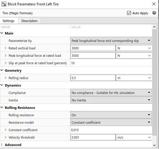
As seen in above image we can model a tire by putting a practical values in parameters block.
- The tires are parameterized by Peak longitudinal force and corresponding slip.
- The other block parameters such as - rated vertical load, peak longitudinal force at rated load and slip at peak force at rated load - are kept with their default values.
- The tire radius is given as 0.3 m.
- The tire inertia is kept as zero. Also, the rolling resistance is given with a constant coefficient of 0.015.
Note : This tire confrigution is same for the all tires
This 2 axle (4 wheel) assembly is now connected to a Vehicle Body simscape block
B.Vehicle Body
Two-axle vehicle with longitudinal dynamics and motion and adjustable mass, geometry, and drag properties
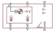
Description
The Vehicle Body block represents a two-axle vehicle body in longitudinal motion. The vehicle can have the same or a different number of wheels on each axle. For example, two wheels on the front axle and one wheel on the rear axle. The vehicle wheels are assumed identical in size. The vehicle can also have a center of gravity (CG) that is at or below the plane of travel.
The block accounts for body mass, aerodynamic drag, road incline, and weight distribution between axles due to acceleration and road profile. Optionally include pitch and suspension dynamics. The vehicle does not move vertically relative to the ground.
The block has an option to include an externally-defined mass and an externally-defined inertia. The mass, inertia, and center of gravity of the vehicle body can vary over the course of simulation in response to system changes.
- Here, the connection H is the mechanical translational conserving port hub.
NF & NR correspond to the output ports for nomral reaction forces on front axle and rear axle wheels respectively.
Connection V represents the actual output translational velocity of the vehicle.
beta is the road inclination angle & W corresponds to the headwind speed (headwind - direction opposite to that of vehicle). - The gross weight is given to be 1000 kg.
- The geometric parameters of the vehicle are given as -
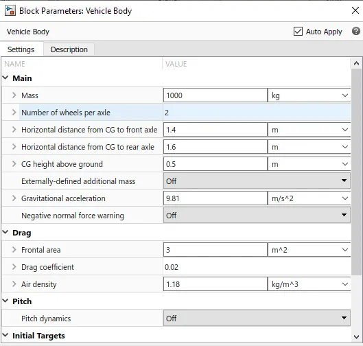
To account for proper drag force on the vehicle, the related parameters are kept as mentioned above
The pitch dynamics for the vehicle are not considered for this simulation.
Now we started to connect the vehicle body to tires
Note : We are going to make a rear wheel drive electrical vehicle.
C. Simple Gear

Description
The Simple Gear block represents a gearbox that constrains the connected driveline axes of the base gear, B, and the follower gear, F, to corotate with a fixed ratio that you specify. You choose whether the follower axis rotates in the same or opposite direction as the base axis. If they rotate in the same direction, the angular velocity of the follower, ωF, and the angular velocity of the base, ωB, have the same sign. If they rotate in opposite directions, ωF and ωB have opposite signs. You can easily add and remove backlash, faults, and thermal effects.
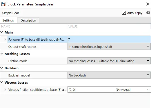
The input for this subsystem is taken as the Rotational speed of the motor. This input is fed to the front axle through a Simple Gear representing the Final Drive Ratio of 7
Note : Higher the gear ratio then the lower speed tracking will be properly performed.
Here, the rotational direction of the output shaft is kep the same as that of the input shaft. Also, no meshing losses and no backlash are considered for the simulation.
The complete subsystem is shown below
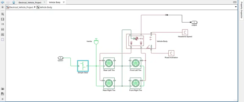
Note : We are not considering the slip of the tire so this ports are remaining disconnected.
2. DC Motor
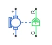
Here, the blue colour corresponds to the electrical side of the motor and the green colour corresponds to the mechanical side.
Description
The DC Motor block represents the electrical and torque characteristics of a DC motor using the following equivalent circuit model:
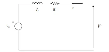
You specify the equivalent circuit parameters for this model when you set the Model parameterization parameter to By equivalent circuit parameters. The resistor R corresponds to the resistance you specify in the Armature resistance parameter. The inductor L corresponds to the inductance you specify in the Armature inductance parameter.
- The connection R represents the Rotor (rotational output) while the connection C is for the Casing (stationary). Thus, the R port is connected to the input of the vehicle subsystem created earlier. The C port is connected to a mechanical rotational reference.
- The + and - terminals of the motor are connected to the motor controller. If these terminals are directly connected to a battery, the required DC motor will run on the rated capacity of the battery. This will eventually result into no control over the DC motor and the vehicle will run at top speed throughout the simulation.
Thus, a motor controller is very much needed. - Here, the motor field type is kept as Permanent magnet and the model parameterization is done by rated load and speed.
The armature inductance and the mechanical parameters are given their default values.
All the other parameters are changed as shown below -
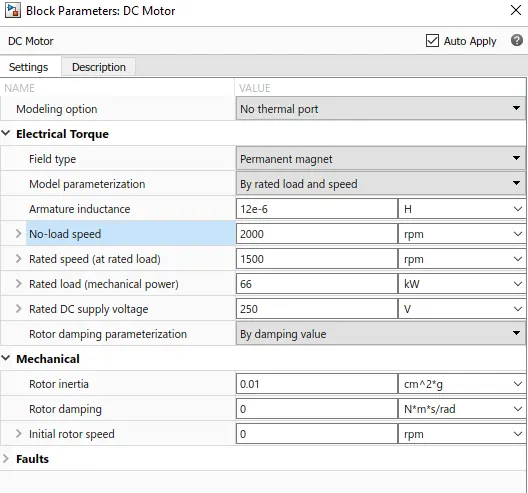
3. Motor Controller
A. H-Bridge Circuit
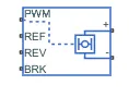
This block represents an H-bridge motor drive. The block can be driven by the Controlled PWM Voltage block in PWM or Averaged mode.
Description
The H-Bridge block represents an H-bridge motor driver. The block has the following two Simulation mode options:
PWM
The H-Bridge block output is a controlled voltage that depends on the input signal at the PWM port. If the input signal has a value greater than the Enable threshold voltage parameter value, the H-Bridge block output is on and has a value equal to the value of the Output voltage amplitude parameter. If it has a value less than the Enable threshold voltage parameter value.
Averaged
This mode has two Load current characteristics options:
-
Smoothed -
Unsmoothed or discontinuous
The Smoothed option assumes that the current is practically continuous due to load inductance.
- In PWM mode, the motor is powered if the PWM port voltage is above the enabled threshold voltage.
- In Averaged mode, the PWM port voltage divided by the PWM signal amplitude parameter defines the ratio of the on-time to the PWM period.
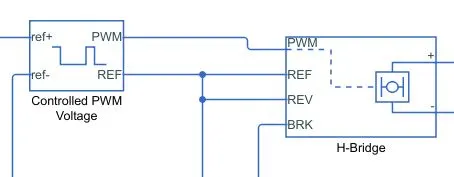
- Connection REF is for the reference input. This combined with the PWM connected will form the pulse input for the H-Bridge.
Here, the REF input is connected to the Electrical Reference (ground). - Connection REV corresponds to the reverse motion of the motor which essentially means, the backward motion of the vehicle.
Here, the backward motion of the vehicle is not accounted for and so, the port is connected to the electrical reference. - Connection BRK is for the braking of the vehicle.
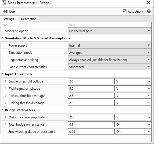
- Since, the PWM mode results in a huge amount of simulation time, Averaged mode is selected for this simulation.
- Load current characteristics are considered to be smoothed here.
- Also, the regenerative braking is anabled for the simulation. This means, when the vehicle starts decelerating, corresponding amount of charge will be fed back to the battery.
Accordingly, the BRK input is connected to a Controlled Voltage Source. This will generate emf corresponding to the intensity of brakes applied and fed the power back to the battery. - The Input Threshold parameters are left with their default values
- The Output Voltage Amplitude of the H-Bridge circuit is given the same value as the rated DC supply voltage of the DC motor.
B. Controlled PWM Voltage

This block is used for providing the proper pulse inputs to the H-Brdige circuit.
Description
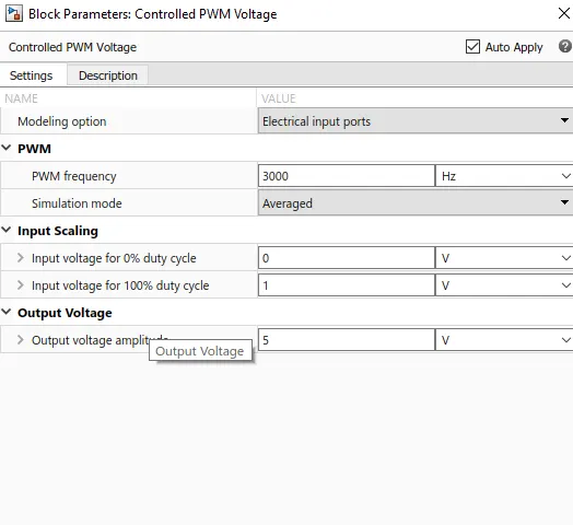
The Controlled PWM Voltage block represents a pulse-width modulated (PWM) voltage source. You can model electrical or physical signal input ports by setting the Modeling option parameter to either:
-
Electrical input ports— The block calculates the duty cycle based on the reference voltage across its ref+ and ref- ports. This option is the default. -
PS input— Specify the duty cycle value directly by using an input physical signal port.
The PWM & REF connections are for the corresponding ports on the H-Bridge circuit.
The 2 reference inputs correspond to the throttle inputs given by the driver. The block generates corresponding pulse width as per the accelerations and brakes apllied by the driver himself. Also, PWM frequency set to 3000 Hz
- The H-Bridge circuit along with the PWM input, together form the motor controller circuit.
4. Longitudinal Driver
Description
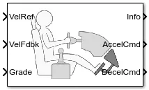
The Longitudinal Driver block implements a longitudinal speed-tracking controller. Based on reference and feedback velocities, the block generates normalized acceleration and braking commands that can vary from 0 through 1. You can use the block to model the dynamic response of a driver or to generate the commands necessary to track a longitudinal drive cycle.
- It is a parametric longitudinal speed tracking controller for generating normalized Acceleration and Braking commands based on reference and feedback velocities.
- The VelRef port is the reference velocity port where the input drive cycle data is fed.
The VelFdbk port corresponds to the feedback velocity. The actual velocity output given by the vehicle body is connected here. By comparing the actual (feedback) velocity with the reference velocity, the driver block generates acceleration and braking signals in order to minimise the error between the two concerned velocities.
Grade corresponds to the grade angle. For this simulation, no inclination is considered and hence, a constant block with value 0 is connected.
Info gives the output for the bus signal for different block calculations like difference in reference vehicle speed and vehicle speed, etc.
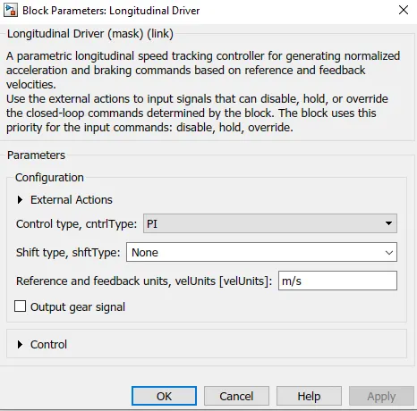
AccelCmd & DecelCmd correspond to the acceleration and deceleration commands generated respectively and are connected to the corresponding ports of the Controlled PWM Voltage block. - Here, the selected control type is PI. Acordingly, the block implements proportional-integral (PI) control with tracking windup and feed-forward gains.
5. Battery

Description
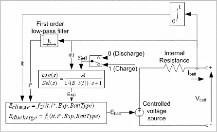
The Battery block implements a generic dynamic model that represents most popular types of rechargeable batteries.
This figure shows the equivalent circuit that the block models.
-
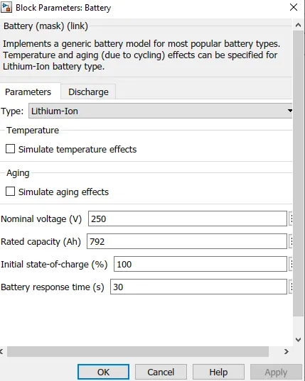
Implements a generic battery model for most popular battery types. Temperature and aging (due to cycling) effects can be specified for Lithium-Ion battery type.
- The selected battery type is Li-ion
- Also the measurment port has SOC , Voltage , Current
- The output of the battery voltage is 250 V and rated capacity is set to 792 Ah
6. Drive Cycle
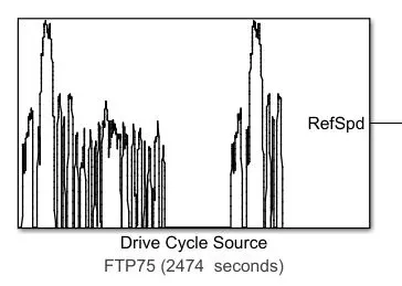
- The Drive Cycle Source block is used to provide the reference speed for the simulation.
- It generates a standard or user-specified longitudinal drive cycle.
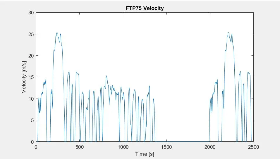
- Here, the selected drive cycle is the standard FTP75.
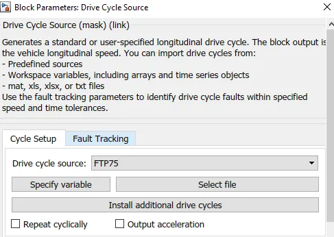
- The plot of the drive cycle is shown below -
The following also used in model for connection purpose and showing the results etc.
1. Scope
2. Bus selector
3. Contolled current source
4. Controlled voltage source
5. Current sensor
6. PS-Simulink converter
7. Simulink-PS converter
8. Display
9. Integer
10. Divide
11. Constant
12. Solver confrigution
13. Powergui
14. Electrical & Mechanical ref.
15. Terminator
Complete Model :
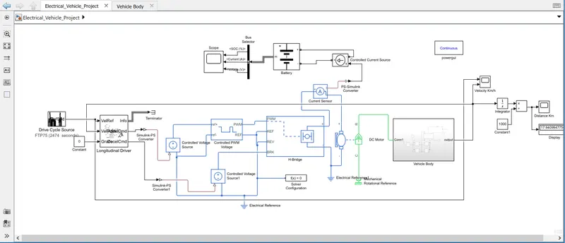
Note : The simulink file is attched with answer body.
- The model is run for simulation for 2474 s which is the total time for which the input drive cycle is defined.
- The distance is calculated by simply time-integration of the vehicle velocity.
RESULTS :
1 Ref. Speed v/s Actual vehicle speed :
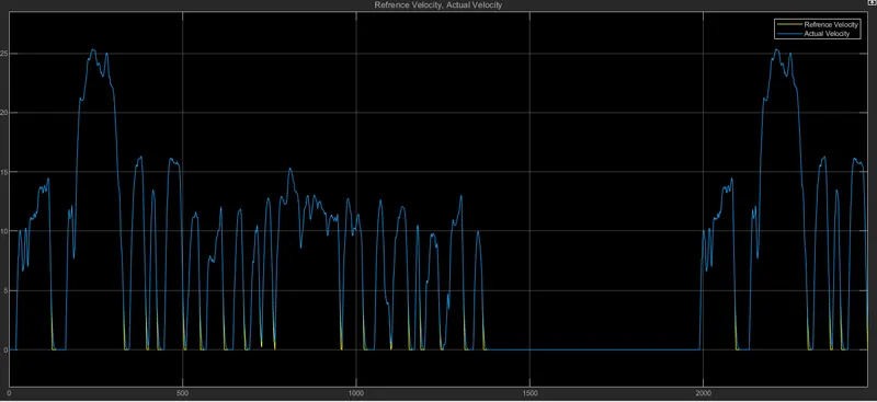
- As can be seen from the above picture, the actual velocity of the vehicle is almost same to the reference drive cycle velocity.
- It means the calculation made by us is corret, the calcuated parameters such as battery voltage and its capacity, motor rated speed and its rated power and the converter parameters etc. are accurate.
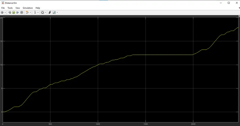
2. Distance Covered :
- The total distance covered by the vehicle is about 17.94 km.
3. Battery Parameters
A. State Of Charge
B. Current
C. Voltage
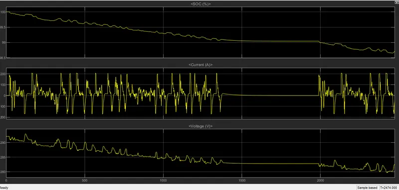
- The State-of-Charge of the battery at the end of simulation run is nearly about 98.5 %.
- This means that the battery is not completely drained at the end and the vehicle can run on the same drive cycle for a few more times before the battery SOC becomes 0. Also, the thing to be noted here is, since we had enabled the regenerative braking for the simulation, the battery SOC increases slightly whenever the vehicle undergoes heavy deceleration.
- As seen in above image the current of the battery increses when there is acceleration in the vehicle and current decreses when there is decleration.
- There is slightly volatge decresing obseved in result.
CONCLUSION :
The model was succesfully run for simulation under the standard FTP75 drive cycle. The results have been properly analyzed.
Also, learnt quite a lot of interesting things like -
- how to model an EV and carry out a real time simulation
- how a motor controller works and what role it plays in the control of the electric motor
- how gear ratio plays important role in tracking the requried low speed.
- different powertrain blocks provided by simulink which can be used to simulate a vehicle model.