Design of an Electric Vehicle using MATLAB-Simulink
Project: Design of an Electric Vehicle
AIM: To create a basic Electric Vehicle model using MATLAB/Simulink
OBJECTIVES:
1. Explain System-level configurations.
2. Explain each model parameters & blocks.
3. Comment on results.
4. Conclusion.
EXPLANATION:
What is an Electric Vehicle?
An electric vehicle (EV) is one that operates on an electric motor, instead of an internal-combustion engine that generates power by burning a mix of fuel and gases. Therefore, such as a vehicle is seen as a possible replacement for current-generation automobile, in order to address the issue of rising pollution, global warming, depleting natural resources, etc. Though the concept of electric vehicles has been around for a long time, it has drawn a considerable amount of interest in the past decade amid a rising carbon footprint and other environmental impacts of fuel-based vehicles.
Types of Electric Vehicles as shown in the below images:
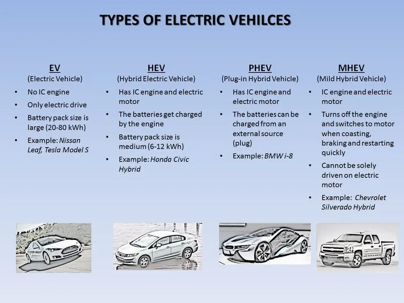
fig. Flow chart of different types of Electric Vehicle
Basic block model of an EV:
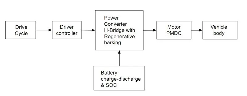
fig. Electric Vehicle architecture
The block diagram above describes the basics architecture of an Electric Vehicle.
Drive cycle: This is the input given to the vehicle. There are different types of drive cycle based on the application we choose. In this vehicle is simulated for acceleration & deceleration for a particular type with the varying speed range.
Driver controller: To drive the drive cycle as per the given condition, a driver controller is present to run the vehicle taking the input and feedback from to move from one place to another.
Power Converter: They are used to process and control the flow of electrical energy by supplying required voltages and current in a form that is optimally suited for the user loads.
Battery: This the powerhouse which supplies the energy required to drive the vehicle.
Motor: It is the rotating device which converts the electrical energy in the form of current and voltage into the mechanical energy at the vehicle through a transmission system.
Vehicle body: This is where the output is achieved via the motor power is transferred to the wheel considering the different forces and resistance and compare with the input drive cycle.
Powertrain Blocksets:
They provide fully assembled reference application models of automotive powertrains, including gasoline, diesel, hybrid, and electric systems. It includes a component library for simulating engine subsystems, transmission assemblies, traction motors, battery packs, and controller models. Also, they provide a standard model architecture that can be reused throughout the development process. It can use it for design tradeoff analysis and component sizing, control parameter optimization, and hardware-in-the-loop testing. And it can customize models by parameterizing components in a reference application with customizing data or by replacing a subsystem with the self-created model.
SYSTEM-LEVEL CONFIGURATION:
(1) Input circuit:
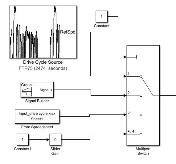
fig. Input signal system blocks
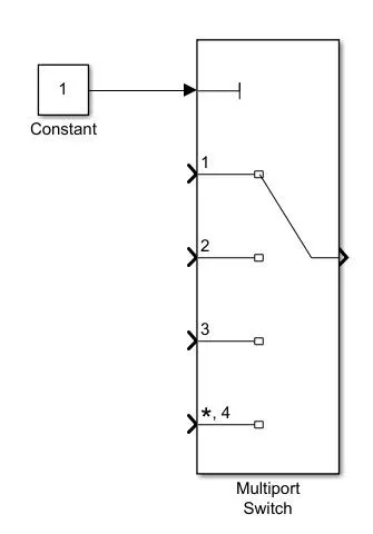
This is the input where the user defines the driver cycle and defines the behaviour of the vehicle movement for a particular time. In this, we have provided 4 different types of inputs to run the simulation of our EV model. A Multiport switch is used to activate the which drive cycle input has to be run for simulation by changing the value of the constant.
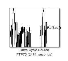
(i) Drive Cycle Source:
It can generate a standard or user-specified longitudinal drive cycle. The block output is the vehicle longitudinal speed. There are different types of predefined drive cycles or can add in MATLAB workspace variables, including arrays and time series objects or spreadsheets.
(ii) Signal Builder:
This block is used to create and generate interchangeable groups of signals whose waveforms are piecewise linear.
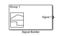
This is defined drive cycle for 200 secs with acceleration at 25th sec and becoming constant after attending top speed of 65 kmph. After 135th sec the vehicle starts deceleration up to the speed of 29 kmph and becomes constant till the end of the drive cycle.
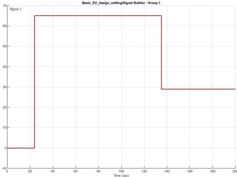
fig. Signal builder drive cycle created for 200 secs
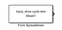
(iii) From Spreadsheet: This block is called out the self-created drive cycle made in Excel sheets and use as an input.
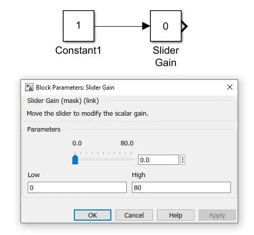
(iv) Slider Gain: This block acts a slider when we can create our own driver cycle while the simulation is running by changing the positon of the slider.
(v) Multiport switch: It passed through the input signals corresponding to the truncated value of the first input. The inputs are numbered top to bottom, where the first input port is the control port and the other input ports are data ports.
(2) Driver Controller:
The input from the drive cycle is attached to VelRef port, the feedback is gained from the vehicle body which acts as feedback signal is connected to VelFdbk. The AccelCmd & DecelCmd are the output signal given for accelerating and braking to the vehicle. A terminator block is connected to Info port as we are not using any bus signals for this model. A constant block is attached to the Grade port as road grade angle is 0 in our case, i.e the vehicle is running at a straight road.
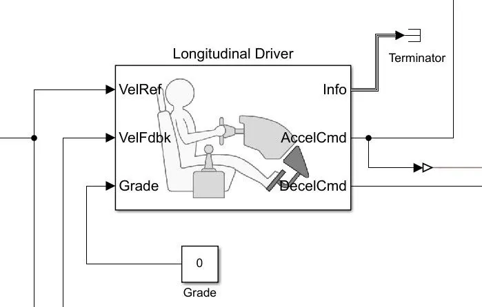
fig. Longitudinal driver system block
Longitudinal driver block: It is a parametric longitudinal speed tracking controller for generating normalized acceleration and braking commands based on reference and feedback velocities. They use the external actions to input signals that can disable, hold, or override the closed-loop commands determined by the block.
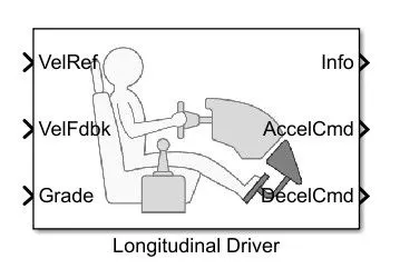
Port:
| Port Name | Description |
| VelRef | Input port for the reference velocity signal |
| VelFdbk | Input port for the feedback velocity signal |
| Grade | Input port for the gradability to the vehicle (road grade angle) |
| AccelCmd | Output port for the acceleration signal command |
| DecelCmd | Output port for the deceleration or braking signal command |
| Info | Bus signal for Gear, clutch, acceleration, etc. |
(3) Power Converter:
This is the main circuit where the input signals are processed and are sent at the output. The electrical power from the battery source is converted into the mechanical output of the DC motor. This block is divided into 3 stages.
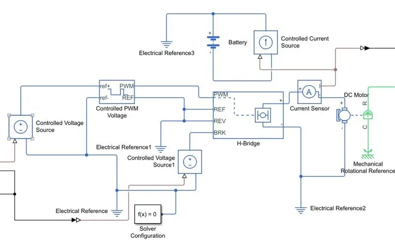
fig. Power converter system blocks
Stage 1: PWM controlled voltage
Stage 2: H-birdge motor drive
Stage 3: Simple DC motor
At stage 1, there are two controlled voltage sources used, one takes the input signals for acceleration from the longitudinal driver's output signal and another is used for deceleration or braking.
At stage 2, the circuit consists of a controller and an H-Bridge. The controlled PWM voltage block receives the input signal from the Acceleration's Controlled voltages source and generated modulated width pulses output for the H-Bridge and which is connected to the positive terminal of the block. The PWM signals are received by the H-Bridge connected to the PWM port of it. The other controlled voltage source is connected to the braking port of an H-Bridge. The reverse port is connected to the ground along with the Reference port. Here we have used selected as Average as the simulation mode to reduce the time for the overall operation.
At stage 3, a DC motor receives the input signal from the H-Bridge and in between them is the current sensor. The rotational motion signal is sent as an output to the motor shaft. A mechanical rotation reference is connected at the constant port.
A battery is attached separately, which is not directly connected to the DC motor but is used for visualization of the SOC of the battery. The signal from the current sensor goes into the controlled current source block. Thus, generating current whenever the vehicle goes into regenerative mode. A subsystem is attached to display the SOC of the battery which is in series with the output signal of the current sensor.
Electrical reference acts as a ground and is connected whenever a ground source is required.
(i) H-Bridge:
This block represents an H-bridge motor drive. The block can be driven by the Controlled PWM Voltage block in PWM or Averaged mode. In PWM mode, the motor is powered if the PWM port voltage is above the Enable threshold voltage. In Averaged mode, the PWM port voltage divided by the PWM signal amplitude parameter defines the ratio of the on-time to the PWM period. Using this ratio and assumptions about the load, the block applies an average voltage to the load that achieves the correct average load current. The Simulation mode parameter value must be the same for the Controlled PWM Voltage and H-Bridge blocks.
If the REV port voltage is greater than the Reverse threshold voltage, then the output voltage polarity is reversed. If the BRK port voltage is greater than the Braking threshold voltage, then the output terminals are short circuited via one bridge arm in series with the parallel combination of a second bridge arm and a freewheeling diode. Voltages at ports PWM, REV and BRK are defined relative to the REF port.
If exposing the power supply connections, the block only supports PWM mode.
PWM - pulse width modulation is the method of reducing average power delivered by an electrical system by effectively chopping it up into discrete parts.
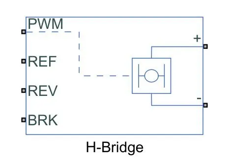
Ports:
| Port Name | Description |
| PWM | Input port for PWM voltage |
| REF | Input port for reference PWM voltage |
| REV | Input port for reverse signal |
| BRK | Input port for brake signal |
Parameters:
Here the power supply is keep at internal and simulation mode as Average (for less run time). Regenerative braking is enable for always.
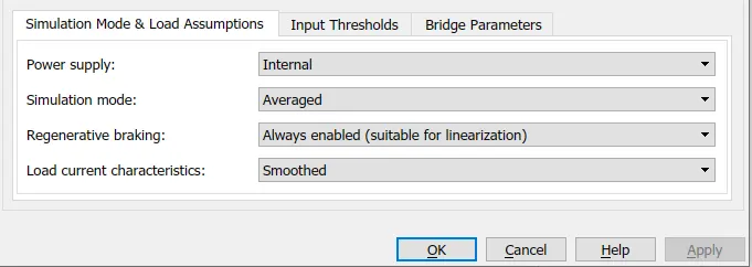
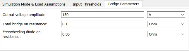
The input thresholds are kept unchanged and in the bridge parameters, the output voltage amplitude is set to 150 V (but depends on the drive cycle0 and the rest of the parameters are unchanged.
(ii) Controlled PWM source:
This block creates a Pulse-Width Modulated (PWM) voltage across the PWM and REF ports. The output voltage is zero when the pulse is low, and is equal to the Output voltage amplitude parameter when high. Duty cycle is set by the input value.
The Simulation mode can be set to PWM or Averaged. In PWM mode, the output is a PWM signal. In Averaged mode, the output is constant with value equal to the averaged PWM signal.
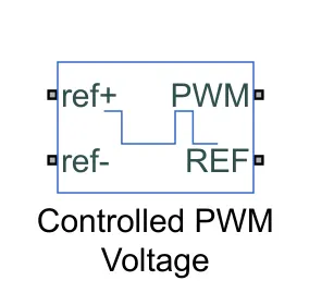
Parameters:
The PWM frequency is set to 1000 Hz and the simulation mode is set to average because it also set as same in an H-bridge.

The input voltage for 100% duty cycle is keep at 5 V as default value.

The output voltage amplitude is set to be at 60 V for more accurate results.

(iii) Controlled Voltage source:
The block represents an ideal voltage source that is powerful enough to maintain the specified voltage at its output regardless of the current passing through it. The output voltage is V = Vs, where Vs is the numerical value presented at the physical signal port.
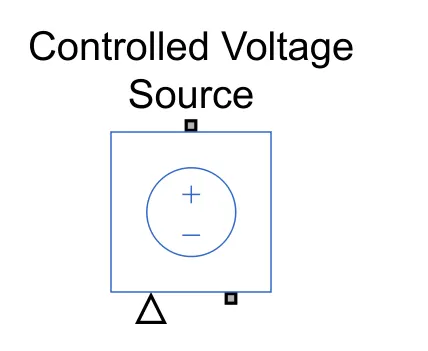
The controlled voltage source block does not have any block parameters of its own. It receives input from the longitudinal driver block and gives output to H-bridge block.
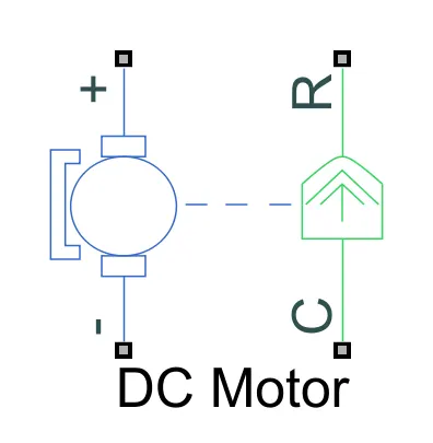
(iv) DC motor:
This block represents the electrical and torque characteristics of a DC motor. It assumes that no electromagnetic energy is lost, and hence the back-emf and torque constants have the same numerical value when in SI units. Motor parameters can either be specified directly, or derived from no-load speed and stall torque. If no information is available on armature inductance, this parameter can be set to some small non-zero value.
When a positive current flows from the electrical + to - ports, a positive torque acts from the mechanical C to R ports. Motor torque direction can be changed by altering the sign of the back-emf or torque constants.
Parameter:
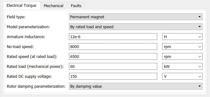
The model parameterization is set as by rated load and speed. The rated DC supply voltage is keep as 150 V which is same as H-bridge's output amplitude voltage. The speed values of the motor at no-load and rated speed is 8000 rpm and 6500 rpm simantenously. And the rated load is at 60 kW (it changes as per the drive cycle). The mechanical and Faults parameter are keep at default.
(v) Battery:
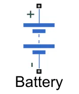
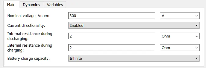
This block models a battery. If you select Infinite for the Battery charge capacity parameter, the block models the battery as a series internal resistance and a constant voltage source. If you select Finite for the Battery charge capacity parameter, the block models the battery as a series internal resistance plus a charge-dependent voltage source defined by:
`V = V_(nom)*(SOC)/(1-beta*(1-SOC))`
where, SOC is the state of charge
`V_nom` is the nominal voltage.
Coefficient `beta` is calculated to satisfy a user-defined data points.
Parameters:
The nominal voltage is set above the DC motor's rated supply voltage and battery charge capacity is keep infinite as there will charging will regenerative braking. Rest other parameters are the default.
(vi) Controlled current source:
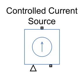
The block represents an ideal current source that is powerful enough to maintain the specified current through it regardless of the voltage across it. The output current is I = Is, where Is is the numerical value presented at the physical signal port.
(vii) Current sensor:
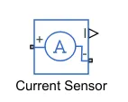
The block represents an ideal current sensor, that is, a device that converts current measured in any electrical branch into a physical signal proportional to the current.
Connections + and - are conserving electrical ports through which the sensor is inserted into the circuit. Connection I is a physical signal port that outputs current value.
(viii) Mechanical rotational reference:
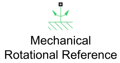
This block represents a mechanical rotational reference point, that is, a frame or a ground. Use it to connect mechanical rotational ports that are rigidly affixed to the frame (ground).
(ix) Electrical reference:
Electrical reference port. A model must contain at least one electrical reference port (electrical ground).

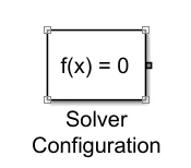
(x) Solver configuration:
it defines the solcer setting to use for simulation when there is connection between simscape blocks and simulink blocks.
(4) Vehicle body
This subsystem represents the 4 wheeler vehicle body with the transmission.
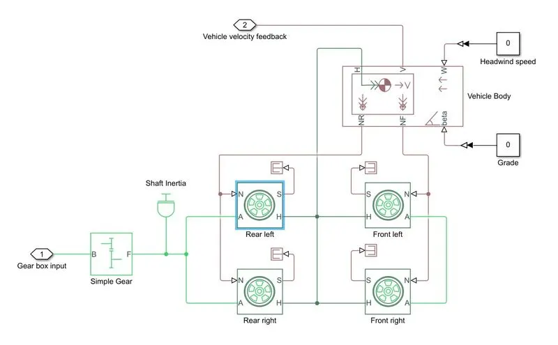
fig. Vehicle body system sub-block
A set of four tire block are used - two for the front axle and two for the rear axle and the required connections are made with the vehicle body block. The normal force signal from the vehicle body block is sent to the normal force input ports of the tires.
The A ports of the tire are the mechanical rotational conserving port and receive mechanical rotational input from the gearbox which receives its input from the DC motor.
The H port of the tire is the mechanical translational conserving port for the wheel hub and is connected to the H port of the vehicle body through which the trust developed by the tire is applied to the vehicle.
Here we are not considering any slip, so an terminator block is connected to all the slip port of each tire. Also, grade angle and wind velocity are not considered.
The input is received from the DC motor to the simple gear block which is then transmitted to the wheel considering the inertia couple at the output shaft.
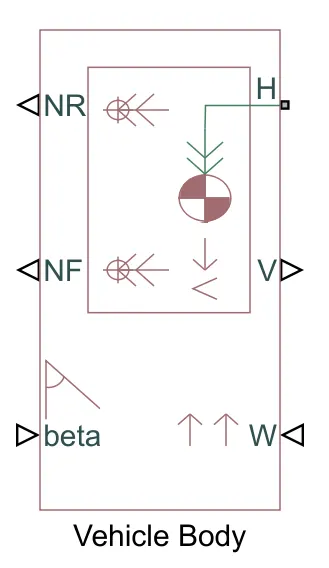
(i) Vehicle body:
The block represents a two-axle vehicle body in longitudinal motion. The block accounts for body mass, aerodynamic drag, road incline, and weight distribution between axles due to acceleration and road profile. The vehicle can have the same or a different number of wheels on each axle. Optionally include pitch and suspension dynamics or additional variable mass and inertia. The vehicle does not move vertically relative to the ground.
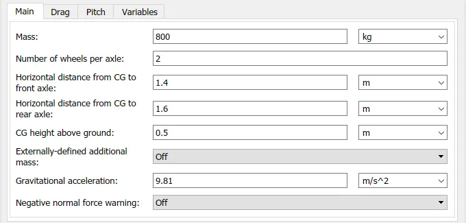
Parameters:
The weight of the vehicle is considered as 800 kg and rest of the parameters are same as default ones.
Ports:
| Port Name | Description |
| H | It is the mechanical translation converting port associated with the horizontal motion of the vehicle body |
| NR | Signal output port for rear normal wheel forces |
| NF | Signal output port for front normal wheel forces |
| V | Signal output port for vehicle velocity |
| Beta | Signal output port for road inclination angle |
| W | Signal output port for headwind speed |
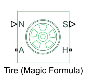
(ii) Tire (Magic formula):
The block represents the longitudinal behavior of a highway tire characterized by the tire Magic Formula. The block is built from Tire-Road Interaction (Magic Formula) and Simscape Foundation Library Wheel and Axle blocks. Optionally, the effects of tire inertia, stiffness, and damping can be included.
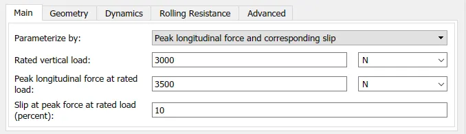
Parameters:
The tire is parameterized by peak longitudinal force and corresponding slip and rest of the parameters are keep as same as default.
Ports:
| Port Name | Description |
| N | Signal input port that applies the normal force acting on the tire |
| A | It is the mechanical rotational conserving port for the wheel axle |
| S | Signal output port that reports the tire slip |
| H | It is the mechanical translational conserving port for the wheel hub |
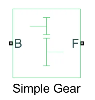
(iii) Simple gear:
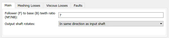
Parameter:
In the we have kept gear ratio as 7. The more the gear ratio the better the speed with more traction power. As torque is directly is directly proportional to the speed. The gear ratio is high at the start of the vehicle as it requires more torque and as the speed increases, torques redues and so as the gear ratio. For our application, the range of gear ratio is from 5-10.
Ports:
| Port Name | Description |
| B | Input signal for mechanical rotational conserving port from DC motor |
| F | Output signal for mechanical rotational conversing port after gear reduction |
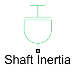
(iv) Shaft inertia:
The block represents an ideal mechanical rotational inertia. The block positive direction is from its port to the reference point. This means that the inertia torque is positive if the inertia is accelerated in the positive direction.
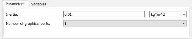
Parameters:
All the parameters are kept as default.
(5) SOC (Stage of Charge):
This will determine the voltage level in the battery at each point of simulation. The output from the current block is received at the input signal of the block and display the characteristic of the battery voltage consumed for the particular drive cycle.
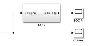
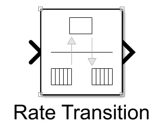
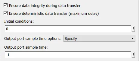
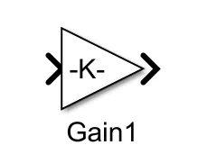
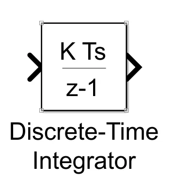
The sub-block of the SOC contains the Rate transition block, gain block and the discrete time ingegrator. The decrease & increase of the battery voltage is have multiple data point which is handle by the rate transistor. Then this converts these data points and calculate the SOC at each point of the drive cycle. The gain block will calculate the values and display on the scope.
The gain is given by
`K = 1/(V__rated*Time)`
where, time is in secs, i.e. 3600 and the multiplication is element-wise.
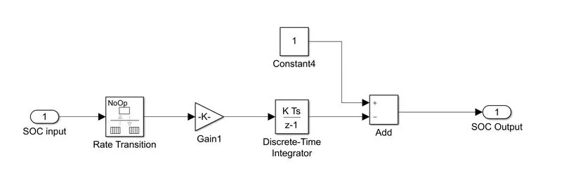
fig. SOC Sub-block system
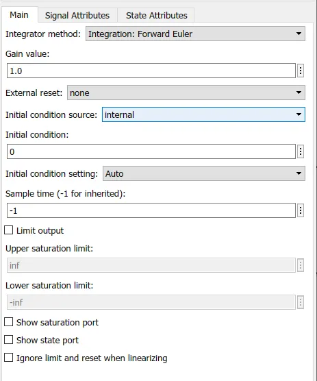
(i) Rate Transistion:
It handles data transfer between different rates and tasks.
Parameters:
(ii) Gain:
(iii) Discrete-time Integrator:
It is the accumulation of the input signals.
Parameters:
(5) Output circuit:
The output of the vehicle body is Velocity which is sent as feedback to the longitudinal driver block and is separately used to calculate the distance travelled by the vehicle through another subsystem - distance calculator.
The velocity signal is first integrated to calculate the distance and then divide by 3600 to convert the distance into km.
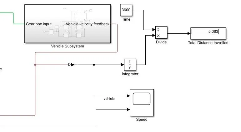
fig. Output system display block
COMPLETE MODEL OF AN EV:
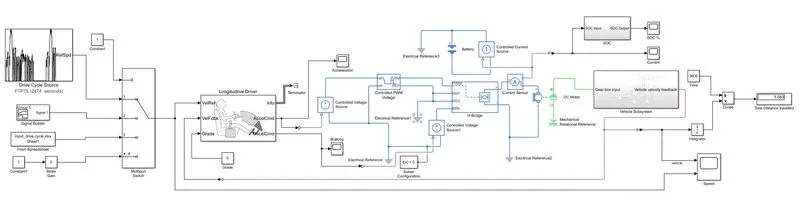
fig. Simulink model of an EV
RESULTS:
The simulations are run for various drive cycles and the results are in the following table.
Simulation Time - It is the time for which the simulation is run. Each drive cycle has its own time duration which needs to be updated in simulation time, each time the drive cycle is changed.
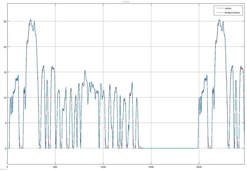
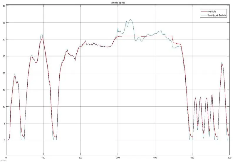
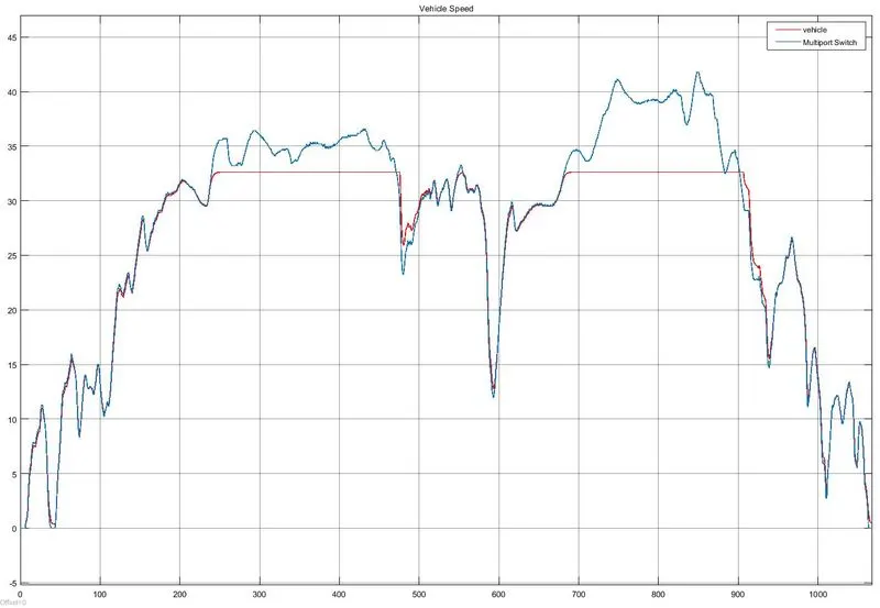
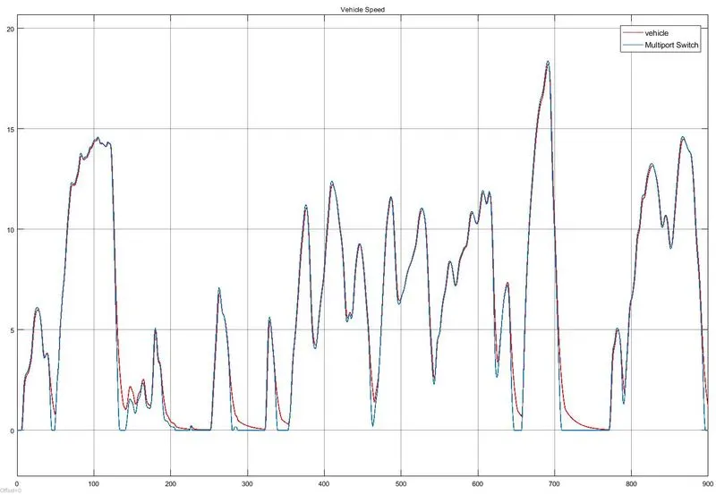
Speed Trace - It is a plot of the reference speed from the drive cycle and the feedback speed from the vehicle body.
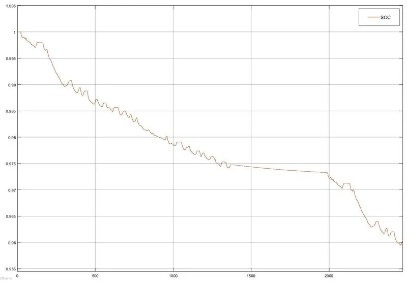
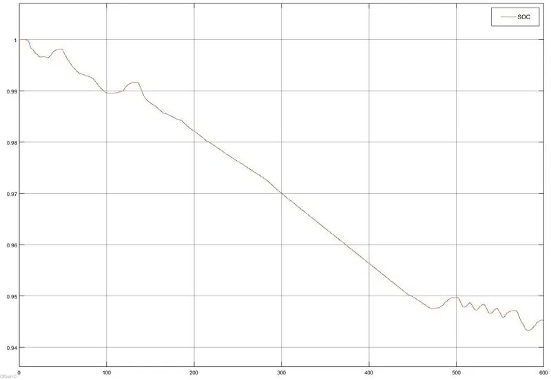
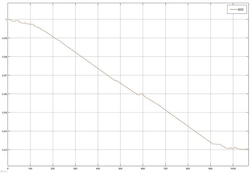
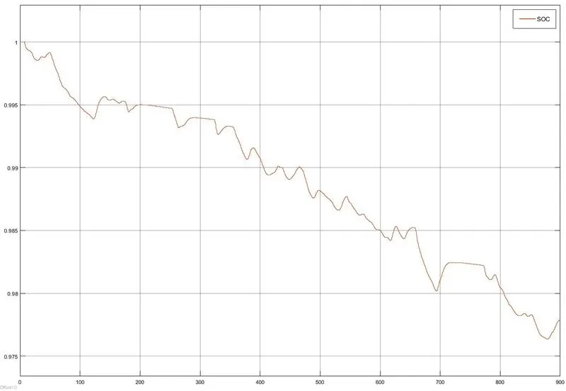
SOC (%) - It is the state of charge of the battery which decreases when the vehicle accelerated and slightly increases when the vehicle decelerates.
Distance Travelled - It is the total distance travelled by the vehicle following a particular drive cycle and its duration.
| Case 1 | Case 2 | Case 3 | Case 4 | |
| Drive Cycle, Simulation Time (sec) | FTP75, 2474 | US06,600 | Artemis Motorway 150kmph, 1068 | World Harmonized Vehicle Cycle (WHVC),900 |
| Vehicle body weight (kg), Frontal area (m2), Drag co-efficient, Rolling resistance | 800,3, 0.4, 0.015 | 800,3, 0.4, 0.015 | 800,3, 0.4, 0.015 | 800,3, 0.4, 0.015 |
| Battery Nominal Voltage (V) | 300 | 300 | 400 | 200 |
| DC Motor Rated load (kW), Rated DC supply voltage (V) | 60, 300 | 75, 200 | 85, 350 | 60, 150 |
| H-Brigde Output voltage amplitude | 300 | 200 | 350 | 150 |
| Distance (km), Top speed (kmph) | 4.97, 25.2 | 3.54,30.8 | 7.77, 32.6 | 1.52,18.2 |
| SOC at end of drive cycle (Initial SOC 100%) | 96 | 94 | 93 | 97 |
| Top speed reached? kWh per km | Yes | No | No | Yes |
Output graphs:
(I) Case 1
(i) Speed Charateristics:
(ii) SOC (%):
(II) Case 2
(i) Speed Charateristics:
(ii) SOC (%):
(III) Case 3
(i) Speed Charateristics:
(ii) SOC (%):
(IV) Case 4
(i) Speed Charateristics:
(ii) SOC (%):
CONCLUSION:
- In the speed trace plots for all the drive cycles which are observed in this study, the feedback speed plot and the reference speed plot overlap each other almost completely but there are regions where both the speeds are different. It is when the vehicle is decelerating.
The reference speed plot falls sharply but the feedback speed does not. This is due to the inertia of the vehicle body. As the inertia of the vehicle body is higher, it takes a longer duration for it to decelerate. That is why the overlapping is not 100%. - The battery's state of charge for each drive cycle can be visualized from the SOC plot. As long as the vehicle is accelerating the SOC is decreasing but as soon as the deceleration starts, the SOC plot goes slightly up. This is because the battery is being charged, due to regenerative braking during deceleration.
DOWNLOAD: EV Simulink model
REFERENCE: