Final Project: Design of an Electric Vehicle
Design of an Electric Vehicle
Aim of the project
To Create a MATLAB model of an Electrical car that uses a battery and a DC Motor.
Objectives of the project
To describe System-level configurations, model parameters, and results of the MATLAB model of EV
Software Used: MATLAB SIMULINK 2020a
Body of the Project
An electric vehicle is a vehicle that uses one or more electric motors (instead of an internal combustion engine) for propulsion. While considering the environment, It is carbon emission-free due to the lack of internal combustion engines. An electric vehicle may have powered through a collector system by electricity from off-vehicle sourced or may be self-contained with a battery, solar panels, fuel cells, or an electric generator to convert fuel to electricity. The efficiency of EV is higher than that of an internal combustion engine. The main components of electric vehicles are the electric motors, batteries for power supply with battery management system(BMS), Vehicle bodies, tires, gear systems,s and driver consoles with control units.
Block Diagram of EV Model
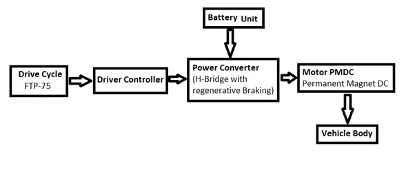
An electrical vehicle runs by an electric motor powered by Batteries and its power is controlled by the driver through a power converter. The power converter used here is H-bridge type. H-Bridge is available as an integrated circuit or can be built from discrete components. H-bridge used here is PWM based one. H-Bridge is built with four switches.S1, S2, S3, and S4 as shown in the figure.
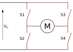
when S1 and S4 are closed and S2and S3 are in an open position means the DC motor will run in Forward direction but in the condition that S1 and S4 are open and S2 and S3 are in closed condition means the motor will rotate in the opposite direction
FTP-75 is the drive cycle used here, The EPA Federal Test Procedure commonly known as FTP75 for the city driving cycle is the series of tests defined by the US Environmental Protection Agency (EPA) to measure tailpipe emission and fuel economy of passenger cars (excluding light trucks and heavy-duty vehicles)
While considering a simple Simulink model of an electrical vehicle main blocks associated with it are
Tires: - Represents the longitudinal behavior of a highway tire characterized by the tire Magic Formula. The block is built from Tire-Road Interaction (Magic Formula) and Simscape Foundation Library Wheel and Axle blocks. Optionally, the effects of tire inertia, stiffness, and damping can be included. Connection A is the mechanical rotational conserving port for the wheel axle. Connection H is the mechanical translational conserving port for the wheel hub through which the thrust developed by the tire is applied to the vehicle. Connection N is a physical signal input port that applies the normal force acting on the tire. The force is considered positive if it acts downwards. Connection S is a physical signal output port that reports the tire slip. Optionally expose physical signal port M by setting Parameterize by to Physical signal Magic Formula coefficients. Physical signal port M accepts a four-element vector corresponding to the B, C, D, and E Magic Formula coefficients.
Image of tire block shown below
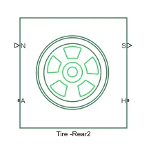
There are four tire blocks are used in this EV Model, and the model designed as a 2wheel drive model so two wheels are assigned for the front and two wheels are assigned for the rear wheels. The Port A, N of two tire rear1 and tire rear 2 are connected and Port A, N of Tire-front1 and Tire-Front2 are connected together, The Port S of tires so it's connected to the PS terminator Block
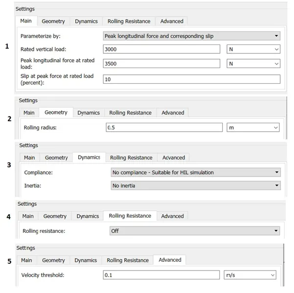
Parameter values of Tire are shown below
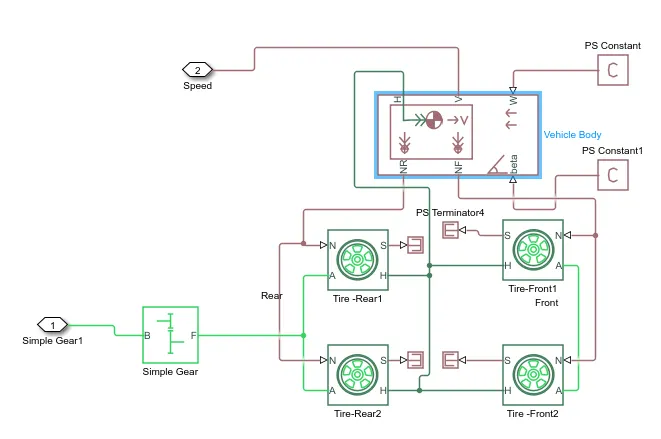
Tire blocks kept under the subsystem named as vehicle body
Vehicle Body: - Represents a two-axle vehicle body in longitudinal motion. The block accounts for body mass, aerodynamic drag, road incline, and weight distribution between axles due to acceleration and road profile. The vehicle can have the same or a different number of wheels on each axle. Optionally include pitch and suspension dynamics or additional variable mass and inertia. The vehicle does not move vertically relative to the ground.
Image of the Vehicle body block
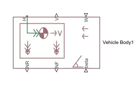
Connection H is the mechanical translational conserving port associated with the horizontal motion of the vehicle body. The resulting traction motion developed by tires should be connected to this port. Connections V, NF, and NR are physical signal output ports for vehicle velocity and front and rear normal wheel forces, respectively. Wheel forces are considered positive if acting downwards. Connections W and beta are physical signal input ports corresponding to headwind speed and road inclination angle, respectively. If the variable mass is modeled, the physical signal input ports CG and M are exposed. CG accepts a two-element vector representing the x and y distance offsets from vehicle CG to additional load mass CG. M represents the additional mass. If both variable mass and pitch dynamics are included, the physical signal port J accepts the inertia of the additional mass about its own CG.
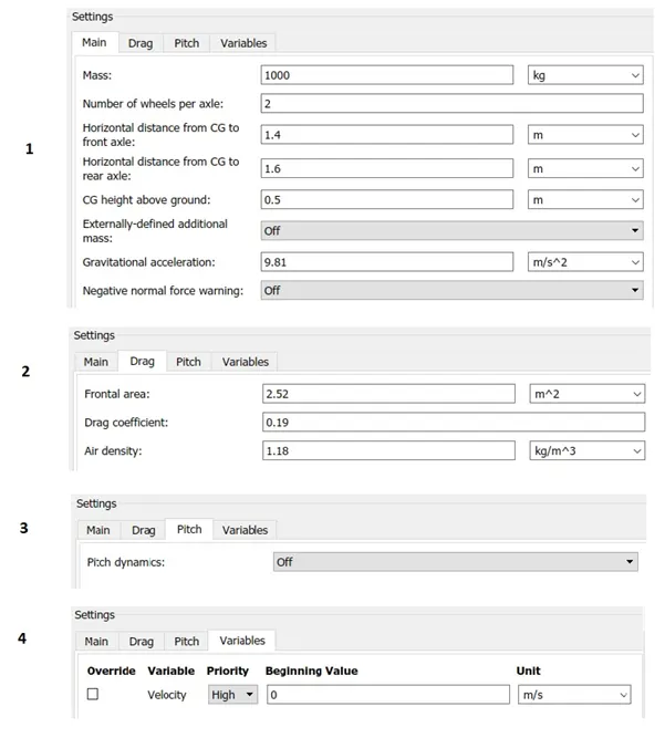
Parameter configuration is shown below
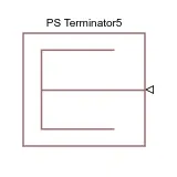
PS Terminator: - Use this block to terminate physical signal outputs. Unconnected physical signal output ports do not generate warnings, but the connection to a PS Terminator can be used to indicate that the signal was not inadvertently left unconnected
Image of PS terminator block shown below
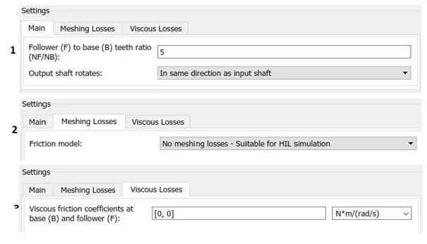
Simple Gear: - Represents a fixed-ratio gear or gearbox. No inertia or compliance is modeled in this block. You can optionally include gear meshing and viscous bearing losses.
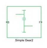
Connections B (base) and F (follower) are mechanical rotational conserving ports. Specify the relation between base and follower rotation directions with the Output shaft rotates parameter. Optionally include thermal effects and expose thermal conserving port H by right-clicking on the block and selecting Simscape block choices to switch between variants.
Parameter settings are shown below
PS Constant: - This block creates a physical signal constant: y = constant, The Constant parameter accepts both positive and negative values. The block output is a physical signal port.
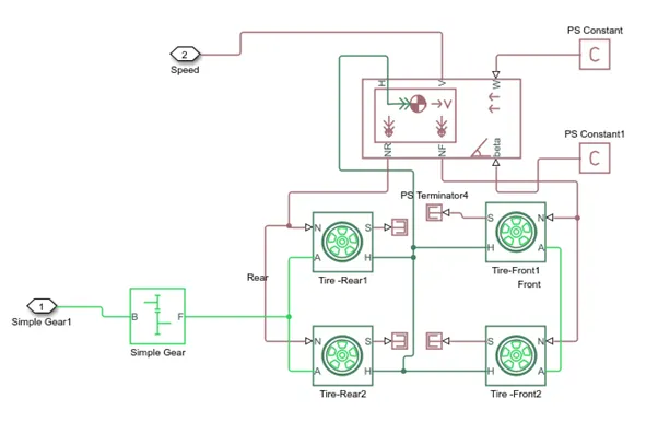
The above-mentioned blocks such as Tires vehicle body, Simple gear, PS constant, PS terminator are belonging to the subsystem Vehicle body and the Simulink model of the subsystem is shown below
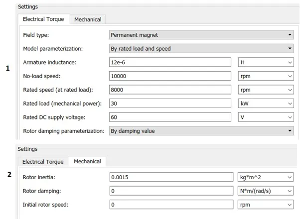
DC Motor: -This block represents the electrical and torque characteristics of a DC motor.
The block assumes that no electromagnetic energy is lost, and hence the back-emf and torque constants have the same numerical value when in SI units. Motor parameters can either be specified directly or derived from the no-load speed and stall torque. If no information is available on armature inductance, this parameter can be set to some small non-zero value. The image is shown below for the block
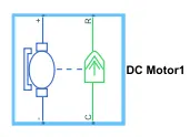
When a positive current flows from the electrical + to - ports, a positive torque acts from the mechanical C to R ports. Motor torque direction can be changed by altering the sign of the back-emf or torque constants. Parameter configuration is shown below
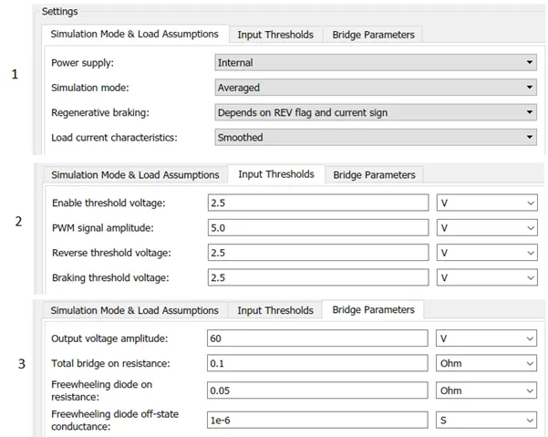
H-Bridge: - This block represents an H-bridge motor drive. The block can be driven by the Controlled PWM Voltage block in PWM or Averaged mode. In PWM mode, the motor is powered if the PWM port voltage is above the Enable threshold voltage. In Averaged mode, the PWM port voltage divided by the PWM signal amplitude parameter defines the ratio of the on-time to the PWM period. Using this ratio and assumptions about the load, the block applies an average voltage to the load that achieves the correct average load current. The Simulation mode parameter value must be the same for the Controlled PWM Voltage and H-Bridge blocks.
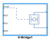
If the REV port voltage is greater than the Reverse threshold voltage, then the output voltage polarity is reversed. If the BRK port voltage is greater than the Braking threshold voltage, then the output terminals are short-circuited via one bridge arm in series with the parallel combination of a second bridge arm and a freewheeling diode. Voltages at ports PWM, REV, and BRK are defined relative to the REF port. If exposing the power supply connections, the block only supports PWM mode. Parameter block settings for the H-Bridge is shown below
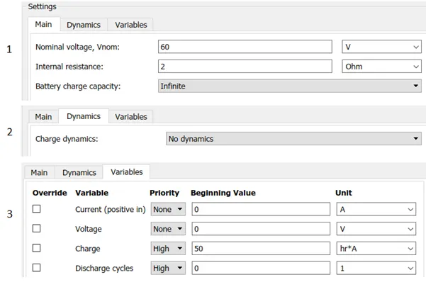
Battery: - This block models a battery. If you select Infinite for the Battery charge capacity parameter, the block models the battery as a series internal resistance and a constant voltage source. If you select Finite for the Battery charge capacity parameter, the block models the battery as a series internal resistance plus a charge-dependent voltage source defined by:
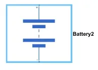
V = Vnom*SOC/(1-beta*(1-SOC)), where SOC is the state of charge and Vnom is the nominal voltage. Coefficient beta is calculated to satisfy a user-defined data point [AH1, V1]. Parameter configuration is shown below
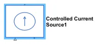
Controlled current Source: -The block represents an ideal current source that is powerful enough to maintain the specified current through it regardless of the voltage across it. The output current is I = Is, where Is is the numerical value presented at the physical signal port.
Current Sensor: -The block represents an ideal current sensor, that is, a device that converts current measured in any electrical branch into a physical signal proportional to the current.
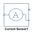
Connections + and - are conserving electrical ports through which the sensor is inserted into the circuit. The connection I is a physical signal port that outputs the current value.
Controlled PWM Voltage: -This block creates a Pulse-Width Modulated (PWM) voltage across the PWM and REF ports. The output voltage is zero when the pulse is low and is equal to the Output voltage amplitude parameter when high. The duty cycle is set by the input value. Right-click the block and select Simscape->Block choices to switch between electrical +ref/-ref ports and PS input u to specify the input value.
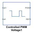
At time zero, the pulse is initialized as high unless the duty cycle is set to zero or the Pulse delay time is greater than zero. The Simulation mode can be set to PWM or Averaged.
Parameter configuration of the controlled PWM voltage is shown below
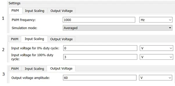
In PWM mode, the output is a PWM signal. In Averaged mode, the output is constant with a value equal to the averaged PWM signal.
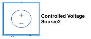
Controlled Voltage source: -The block represents an ideal voltage source that is powerful enough to maintain the specified voltage at its output regardless of the current passing through it. The output voltage is V = Vs, where Vs is the numerical value presented at the physical signal port.
Terminator: - Used to "terminate" output signals. (Prevents warnings about unconnected output ports.)
Longitudinal driver: - A parametric longitudinal speed tracking controller for generating normalized acceleration and braking commands based on reference and feedback velocities.
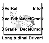
Use the external actions to input signals that can disable, hold, or override the closed-loop commands determined by the block. The block uses this priority for the input commands: disable, hold, override
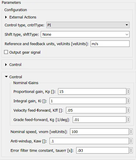
Constant: -Output the constant specified by the 'Constant value' parameter. If 'Constant value' is a vector and 'Interpret vector parameters as 1-D' is on, treat the constant value as a 1-D array. Otherwise, output a matrix with the same dimensions as the constant value.
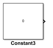
Parameter value configured based on the output constant value required here considered grade is zero so the value of constant kept as zero another constant block is used for the conversion of speed in hour format to sec format instead of constant value selection of zero in the parameter setting changes to 3600 in that block.
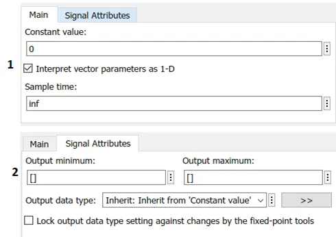
Drive cycle source: -Generates a standard or user-specified longitudinal drive cycle. The block output is the vehicle's longitudinal speed. You can import drive cycles from:
- Predefined sources, The selected drive cycle is FTP75.
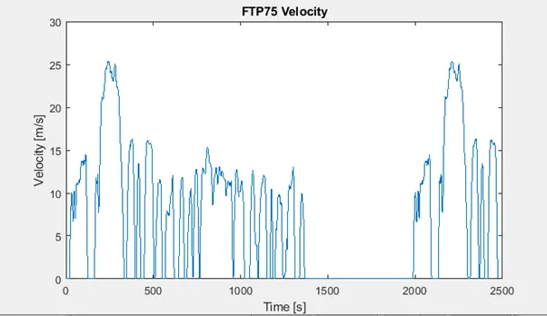
PS- Simulink converter: - Converts the input Physical Signal to a Simulink output signal.
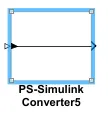
The unit expression in the 'Output signal unit' parameter must match or be commensurate with the unit of the Physical Signal and determines the conversion from the Physical Signal to the Simulink output signal. 'Apply affine conversion' check box is only relevant for units with offset (such as temperature units).
Simulink-PS converter: - Converts the Simulink input signal to a Physical Signal.
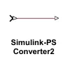
The unit expression in the 'Input signal unit' parameter is associated with the Simulink input signal and determines the unit assigned to the Physical Signal. 'Apply affine conversion' check box is only relevant for units with offset (such as temperature units). If the selected solver requires input derivatives, you can either provide them explicitly through additional signal ports or turn on input filtering to calculate time derivatives. The first-order filter provides one derivative, while the second-order filter provides the first and second derivatives. For piecewise-constant signals, you can also explicitly set the input derivatives to zero.
Solver Configuration: - Defines solver settings to use for simulation.
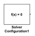
Parameter settings are shown below
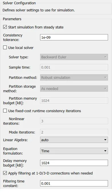
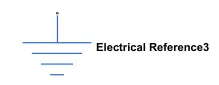
Electrical reference: - Electrical reference port. A model must contain at least one electrical reference port (electrical ground).
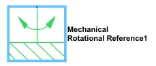
Mechanical Rotational reference: - This block represents a mechanical rotational reference point, that is, a frame or aground. Use it to connect mechanical rotational ports that are rigidly affixed to the frame (ground).
Ideal Rotational Motion sensor:- The block represents an ideal mechanical rotational motion sensor, that is, a device that converts an across variable measured between two mechanical rotational nodes into a control signal proportional to angular velocity or angle. The sensor is ideal since it does not account for inertia, friction, delays, energy consumption, and so on.
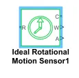
Connections R and C are mechanical rotational conserving ports and connections W and A are physical signal output ports for velocity and angular displacement, respectively.
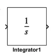
Integrator: - Continuous-time integration of the input signal.
Divide: - Multiply or divide inputs. Choose element-wise or matrix product and specify one of the following: a) * or / for each input port. For example, **/* performs the operation 'u1*u2/u3*u4'.
- b) A scalar value specifies the number of input ports to be multiplied. For example, 2 performs the operation 'u1*u2'.
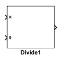
If there is only one input port and the Multiplication parameter is set to Element-wise (.*), a single * or / collapses the input signal using the specified operation. However, if the Multiplication parameter is set to Matrix (*), a single * causes the block to output the matrix unchanged, and a single / causes the block to output the matrix inverse
Display: - Display input values. If the incoming signal is of type string, the 'Numeric display format' parameter selection does not affect the display of the string
Scope: - Scope Block is used to plot the input given to the scope with time on X-axis
MATLAB Simulink model of EV is shown below
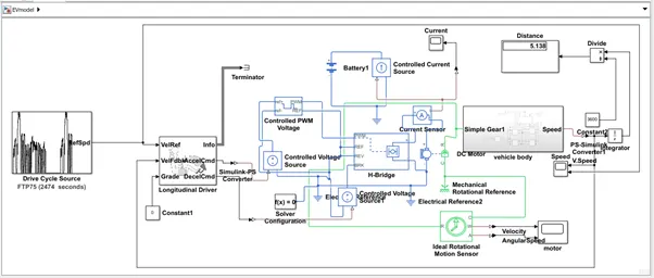
The subsystem vehicle body is created initially by using the blocks of the vehicle body, tires, Simple Gears, PS terminator, and PS constants parameter configuration done as in the block sets shown two Tires which are considered as the front wheel and its N port connected to the NF Port of the Vehicle body block, N ports of another two tires are connected to the NR for the rear wheel, and the slip Port is connected to the PS terminator then road inclination angle beta and wind speed connected to PS constants Separately. A vehicle designed is a rear-wheel-drive so the gear system is connected. V Port of the vehicle body is connected to tap the vehicle speed. To avoid complications of model wheel gear and vehicle body kept under the subsystem.
There are two ports are there for the subsystem Vehicle body one is for tapping the velocity of the vehicle and the other one is connected to the R port of the DC Motor. The DC Motor Provides Rotational Force to the Gear to deliver motion to the vehicle. The DC Motor speed is controlled by a controlled PWM Voltage which will be connected to the DC Motor through the H-Bridge Drive, A current sensor is connected to measure current usage from the Battery to Run the motor. The Drive H-bridge is triggered by the PWM voltage source, +ref Port Voltage source of the controlled PWM Voltage is connected to a controlled voltage source from this based on this controlled Voltage source the Controlled PWM Voltage block produces a PWM output to the H-Bridge PWM port.
Here the Drive Cycle Source Provides the Drive cycle data to the Longitudinal driver block, FTP75 (2474 Seconds) is the selected driving Cycle here. Reference speed Port of Drive Cycle is connected to the Velocity reference of the longitudinal driver block. In the Longitudinal driver block, there are 6 Ports are there VelRef for Velocity reference, VelFdbk for velocity feedback, AccelCmd for Acceleration command, DecelCmd for Deceleration command, and an info block. Here the given Drive cycle (FTP75) will provide the acceleration-deceleration and all values by the velocity reference curve from the drive cycle data.
All electrical Blocks are connected to an electrical reference and the mechanical device (DC Motor) is connected to the Mechanical rotational reference.
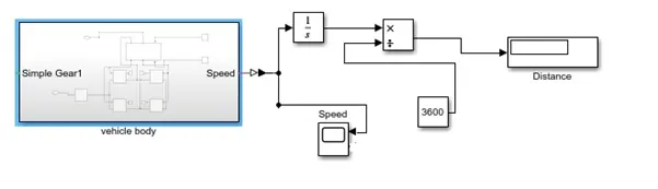
Distance traveled: -We know the velocity of the vehicle at a time interval is the distance traveled in a specified interval of time, which means distance can be calculated from the velocity of the vehicle by integrating velocity with respect to time. Here the integrated value is divided by 3600 to convert m/h to m/sec
Results
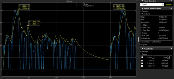
Speed of Vehicle:- From the port of the vehicle body block we can tap the velocity of the vehicle and the drive cycle speed command was given to the vehicle.
The speed Vs time curve of the vehicle is shown below
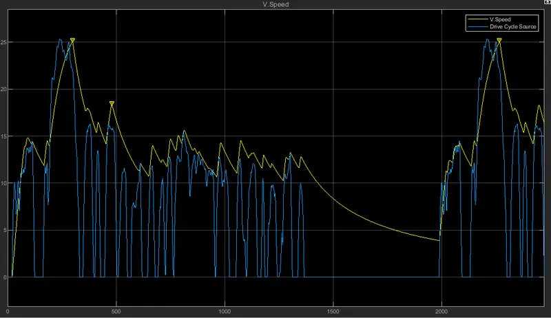
The differences are there in the plot is due to the regenerative braking process it takes time to stop the vehicle motion, that's, why there is a time delay for action, and the vehicle speed, will not increase suddenly it will increase slightly based on the motoring condition by the dc motor by the effect of the converter and its controller.
The blue-colored plot indicates the drive cycle and the yellow-colored one indicates the actual vehicle speed. The peak value of the drive cycle plots is 25.35
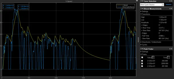
Peak Values of actual vehicle speed are 25.03.
The plot for battery current is shown below
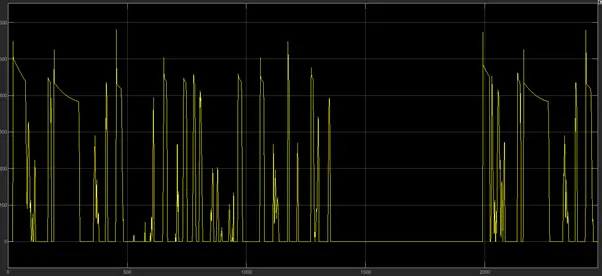
the above-shown plot just measuring the current used during the time of vehicle running condition, Due to the regenerative braking the battery get charged during the time of braking or in the time of power supply to the motor getting disconnected
Output Curve of Ideal rotational motion sensor is shown below
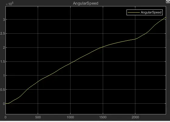
The plot shown above is to identify the motor condition such as its running or not it is tapped from the ideal rotational motion sensor.
Conclusion
The MATLAB model of an electrical vehicle is created and simulated. From the simulation, we can conclude that the velocity of a vehicle varies with various Parameters like frontal area, motor power battery capacity, the converter factors, etc.