Final Project: Design of an Electric Vehicle

AIM -

• To Create a MATLAB model of an electric car that uses a battery and a DC motor.
• To Choose suitable blocks from the Powertrain block set
• To prepare a report about your model including the following:

  1. System-level configurations

  2. Model parameters

  3. Results

  4. Conclusion

SOFTWARE USED -

• MATLAB SIMULINK

ELECTRIC VEHICLE -

Basically, there are two types of electric vehicles

• Pure Electric vehicle
• Hybrid Electric vehicle

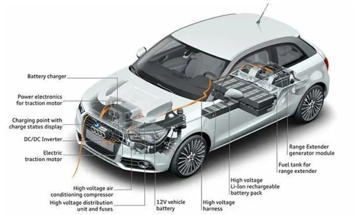
Pure Electric Vehicle - Pure Electric vehicles run only on electricity. Typical pure electric vehicle mileage ranges from 130km/charge to 160km/charge. Few Luxury models range to 1000km/charge such as the tesla roadster.

Pure electric vehicle block diagram -

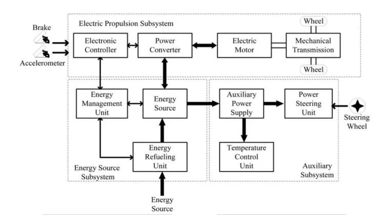The above block diagram is classified into three categories: electric propulsion subsystem, energy source subsystem, auxiliary subsystem. Where electric propulsion system consists of an electronic controller, power converter, motor, transmission system with wheels and energy source subsystem consists of energy source(battery), Energy management unit(battery management system), energy refuelling unit (rectifier) and auxiliary subsystem consists of power steering along with steering wheel, auxiliary power supply, temperature control unit.

We can control the electric vehicle with brake, accelerator, steering wheel, where brake and accelerator input is given to the control unit and steering input is given to the power steering unit.

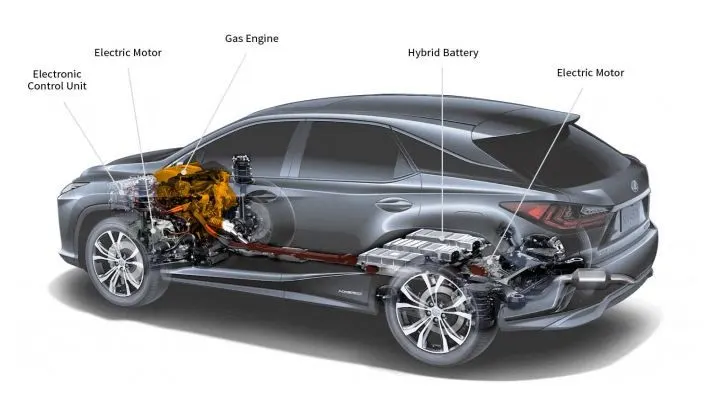
Hybrid electric vehicle - Hybrid electric vehicles are powered by an internal combustion engine and an
electric motor, which uses energy stored in batteries.HEVs are classified into three categories such as series HEV, parallel HEV, and combination HEV.

Basic Architecture of Hybrid Electric Vehicle -

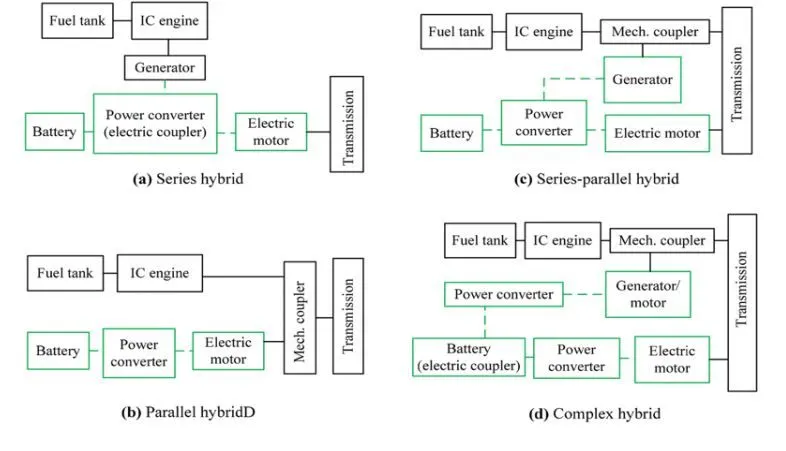There are four architectures for hybrid electric vehicles such as series hybrid, parallel hybrid, series-parallel hybrid, complex hybrid.

Series hybrid - In the above Figure (a), we can see that the series HEV is composed of ICE, generator, power converter, motor, and battery. There is no mechanical connection between ICE and transmission. IC engine uses the fuel from the fuel tank to create mechanical rotation, this is mechanical rotation is converted to electric power using a generator, electric power generated using a generator is sent to power converter to which battery and electric motor is connected. To control the speed of the motor, a controller is used and an electric motor is connected to transmission so that the electric vehicle moves.

Parallel hybrid - In the above Figure (b), we can see that the parallel HEV allows both the electric motor and ICE to deliver power in parallel to drive the vehicle. In parallel HEV, both ICE propulsion and electric motor propulsion is synchronised concerning driving cycle and control strategies.

Series - parallel hybrid -In the above Figure (c) we can see that the combination HEV incorporates the features of both series and parallel HEV, an additional mechanical connection between ICE and transmission is added compared with the series hybrid, and also an additional generator between ICE and power converter is added compared with the parallel hybrid.

SIMULATION MODEL OF ELECTRIC VEHICLE -

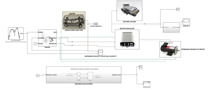The above image is a simulation diagram of an electric vehicle with a permanent magnet DC motor controlled by an H bridge controller. Before explaining the working of the above simulation, let me list out and explain the components used in this simulation.

Components used -

• Driving cycle
• Longitudinal Driver
• Vehicle body
• Tire(Magic formula)
• Simple gear
• H-Bridge
• Controlled PWM voltage
• current sensor
• controlled voltage sensor
• controlled current sensor
• DC motor
• Battery

DRIVING CYCLE -

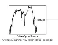The Drive Cycle Source block generates a standard or user-specified drive cycle. It is typically a curve formed by the vehicle speed (longitudinal) with respect to time. Initially, there are only a few drive cycles present, if we need more driving cycles, we can install few more.

The Common Artemis Driving Cycles (CADC) are chassis dynamometer procedures created as part of the European Artemis (Assessment and Reliability of Transport Emission Models and Inventory Systems) project, based on a statistical analysis of a huge database of real-world driving patterns in Europe. There are three driving schedules included in the cycles: (1) urban, (2) rural road, and (3) highway. The Motorway cycle comes in two models, with top speeds of 130 and 150 km/h.

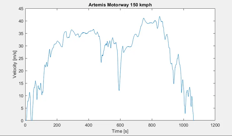The driving cycle that I have used in this project is the Artennis motorway 150kmph(1068 seconds). For this Drive Cycle, it takes 1068 seconds to complete the entire setup and so that's why the entire model is also run for 1068 seconds.

LONGITUDINAL DRIVER -

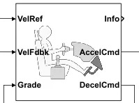Driver behaviour is an essential part of vehicle dynamics and control research. It is also a critical foundation for the closed-loop evaluation of vehicle control stability and the creation of a vehicle aided driving system. The driver's behaviour when controlling the vehicle is a procedure that involves simultaneously altering the vehicle's direction and speed. This allows the vehicle to drive in a safe manner in accordance with the Driver's desire. Driving behaviour consists mostly of two components: vehicle direction control and vehicle speed control.

The Longitudinal Driver block implements a longitudinal speed-tracking controller. Based on reference and feedback velocities, the block generates normalized acceleration and braking commands that can vary from 0 through 1. we can use the block to model the dynamic response of a driver or to generate the commands necessary to track a longitudinal drive cycle.

VEHICLE BODY -

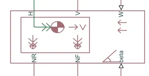This block displays the body of a two-axle vehicle in longitudinal motion. This block allows you to have the same or a varied number of wheels on each axle, as well as include pitch and suspension dynamics or additional changeable mass and inertia. In reaction to system changes, the mass, inertia, and centre of gravity of the vehicle body can alter in simulation.

In the above block,

V = Actual velocity of the vehicle

W = headwind speed

NF - frontal axle normal force

NR - Rear axle normal force

We can assign vehicle mass, The number of wheels per axle, Horizontal distance from the front and rear axle.

TIRE (Magic formula) -

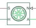It represents the longitudinal behaviour of a highway tire characterized by the tire magic formula. The block is built from Tire-Road interaction(Magic Formula) and Simscape foundation library wheel and axle blocks. Additionally, the effects of the tire inertia, stiffness and damping can be included as per requirements. To increase the fidelity of the tire models, you can specify properties such as tire compliance, inertia and Rolling resistance. However, these properties will increase the complexity of the tire models and can increase the simulation time. One has to ignore the tire compliance and the inertia if simulating the model in real-time or if preparing the model in hardware-in-loop(HIL) simulation.

SIMPLE GEAR -

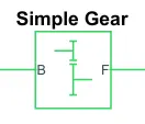It represents a fixed-ratio gear or gearbox. It does not include any options regarding Inertia or Compliance. This block gives the options for including gear meshing and vicious bearing losses.

H-BRIDGE -

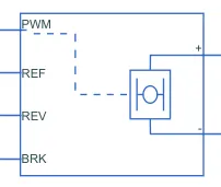It is an electronic circuit that helps us to apply voltage to load in both directions.

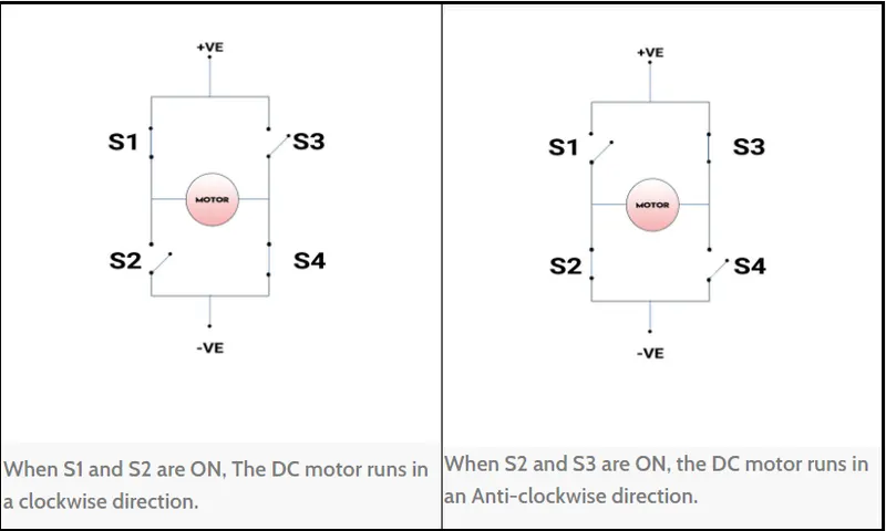The H-Bridge block in Matlab performs the same function as mentioned before and is eventually driven by the Controlled PWM Voltage block in Average Mode as required by the project. The ratio of the on-time to the PWM period in Average Mode is defined by the PWM port Voltage divided by the PWM signal amplitude parameter. The block applies the average voltage to the load to get the proper average load current using this ratio and assumptions about the load. The Simulation mode parameter value for the Controlled PWM Voltage and the H-Bridge block must be the same. The output voltage polarity is reversed if the REV port voltage is greater than the Reverse Threshold Voltage. If the BRK port voltage exceeds the Braking Threshold Voltage, the output terminals are short-circuited through one bridge arm in series with the parallel combination of the second bridge arm and the freewheeling diode. The load current characteristics are adjusted to Smoothed rather than Discontinuous for Average Simulation Mode.

DC MOTOR -

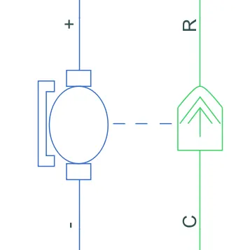This block displays the DC Motor's electrical and torque characteristics. In the assumption that there is no electromagnetic energy is wasted, the back emf and torque constants have the same numerical value as in SI Units. The motor's characteristics are either chosen directly or calculated from the no-load speed and stall torque. Positive torque acts from the mechanical C to R ports when positive current flows from the electrical positive to negative ports. Motor The sign of the back-emf or torque constants can be adjusted to vary the torque direction. The type of Motor chosen is the Permanent Magnet Type so that it resembles the BLDC type of Motor which is most commonly used in the Electric Vehicle.

BATTERY -

The Battery block represents a simple battery model.

EXPLANATION OF THE SIMULATION -

Designing an electrical vehicle has several parts, such as vehicle body dynamics with tyre attached, motor controller, SOC calculation, Distance travelled calculation.

Vehicle dynamics -

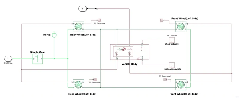The Above simulation consists of a vehicle body block and tire block. Nf(Frontal axle normal force) and Nr(rear axle normal force) of vehicle body block are connected to the hub of each tyre. The axles of the tyres are interconnected. The normal force port of the tyres is interconnected. if we want to specify headwind speed we can specify using a physical constant block. The axle of the front tyres(front-wheel drive) or back tyres(back wheel drive) is connected to the follower port of the simple gear box. Now, the base port of the simple gearbox is connected to the motor rotating part(aka rotor). the motor is powered by using the internal battery present in the H bridge converter. we can also use an external battery option. To control the voltage supplied to the motor and to take reverse and to use regenerative braking we need a controller, control that I have used is an H bridge controller.

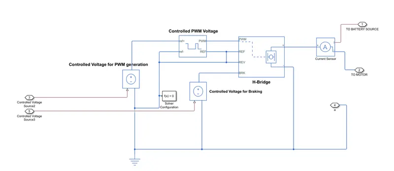The above image is the Motor controller setup. the switching signals are given to H-Bridge using controlled PWM voltage which will actually apply pulses and based on these pulses, from the fixed battery voltage, the variable will be available to the motor. H-bridge block also has a reverse port, break port. as the name implies reverse port is used to reverse the direction of the motor and brake port is used to stop the motor rotation. To accelerate and stop the vehicle, a controlled voltage source is connected controlled PWM voltage block and brake port in the vehicle body block.

The acceleration and braking signal is given taken using driving cycle data and if we want to manually apply acceleration or brake we can use slider gain block. To use this signal and apply it we need a longitudinal driver block, which actually compares the reference velocity from the driving cycle and actual velocity from the vehicle body block, if reference velocity is less than the actual velocity then the longitudinal driver gives an acceleration signal to match the actual velocity, and if actual velocity is greater than reference velocity the longitudinal driver block applies the brake to match the reference velocity.

This way we can control the electric motor attached to the electric vehicle, therefore ultimately we are controlling the electric vehicle.

To estimate the state of charge of the electric vehicle,

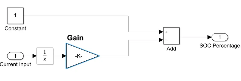To find the SOC of the vehicle I have taken the actual velocity the vehicle is travelling and integrate it with a gain of 1/(140*3600) and add them with constant 1. we get the SOC % curve of the electric vehicle.

To calculate the distance travelled by the vehicle.

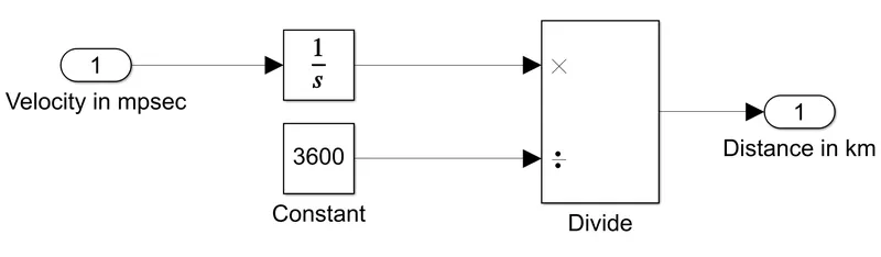To calculate the distance travelled by the vehicle, I have taken the actual vehicle velocity and integrate it we get the distance travelled in metre/sec and to convert that metre/sec to km/s we divide that value with 3600.

RESULTS - I executed the aforementioned drive cycle on my EV model and recorded the results from the speed, current, and SOC scopes. The display block also measures the vehicle's distance travelled during the drive cycle. The run time was modified prior to simulation based on the driving cycle time of 1068secs.

VELOCITY CURVE -

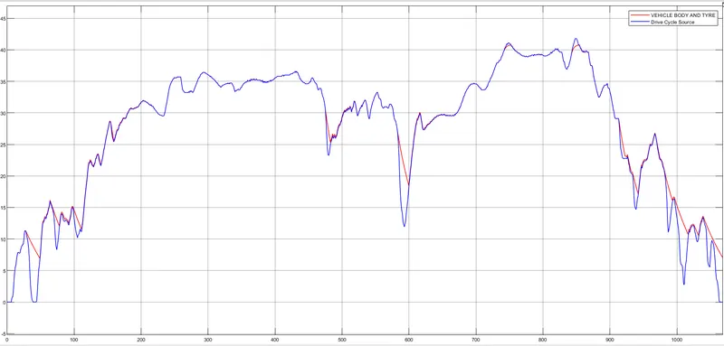The above graph is the combination of both reference and actual velocity graph, the red line is the actual velocity curve where as blue is the reference velocity curve. As explained earlier, the longitudinal driver compares these two curves and if the Actual velocity curve is greater than the reference velocity curve the longitudinal driver block, gives brake signal to the motor controller and if the reference velocity curve is greater than the actual velocity curve then longitudinal driver block gives accelerator signal to the motor controller. That's the reason why these two curves are coinciding. In some places, we can see that the red line and blue line are not coinciding, the reason for that is signal from reference might have been sudden, so the actual vehicle speed takes some time to slow down.

STATE OF CHARGE -

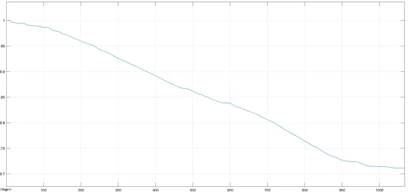The rate at which the battery will get discharged over the entire Driving Cycle is shown in the above figure. This curve depicts the amount of charge remaining in the battery at the end of the Driving Cycle, which is around 0.72 or 72 per cent.

Those little upward spikes in the curve are caused by the phenomena of Regenerative Braking, which occurs as the vehicle decelerates and power is given back to the battery via the reverse rotation of the DC Motor.

DISTANCE TRAVELLED -

From the above image, we can say that distance travelled by the vehicle is 8.376km in 1068 seconds.(i.e the vehicle travelled 8.3 km in 17 minutes approx.).

CONCLUSION -

The EV models are developed using SIMULINK software with appropriate block components and the model was simulated with the Artemis highway 150kmph industry cycle. The simulation generated the results of the speed of the vehicle, battery current and charge status as well as the trip distance during the simulation time. The EV model has a mileage of 8.306kms and that appears to be a reasonable number based on the driving cycle of Artemis. Up to 75 per cent of the total battery charging was efficiently drained. This model also includes features like regenerative braking. Thus the EV design model is successfully implemented with detailed discussion and implementation of the given objectives related to the project.

MODEL - https://drive.google.com/file/d/1pI1u53i6NgloZQXEe0jhhv6gBfp7pZtW/view?usp=sharing