Drag force on a cyclist

Aim: To calculate the Drag force acting against a cyclist and to plot its characteristics using MATLAB

Governing Equation: Fd=0.5.cd.ρ.A.v2">Fd=0.5.cd.ρ.A.v2

where,

Fd=Dragforce(N)">Fd=Dragforce(N)

ρ=Density(kgm3)">ρ=Density(kgm3)

cd=Dragcoefficient(unit≤ss)">cd=Dragcoefficient(unit≤ss)

V=velocity(ms)">V=velocity(ms)

A=FrontalArea(m2)">A=FrontalArea(m2)

Objective: To calculate the Drag force and plot characteristics of the following

• Velocity vs drag force
• Drag coefficient vs drag force for different shapes

Theory : In fluid dynamics, drag (sometimes called air resistance, a type of friction, or fluid resistance, another type of friction or fluid friction) is force acting opposite to the relative motion of any object moving with respect to a surrounding fluid. This can exist between two fluid layers (or surfaces) or a fluid and a solid surface. Unlike other resistive forces, such as dry friction which are nearly independent of velocity, drag forces depend on velocity.

Drag force is proportional to the velocity for a laminar flow and the squared velocity for a turbulent flow. Even though the ultimate cause of a drag is viscous friction, the turbulent drag is independent of viscosity. Drag forces always decrease fluid velocity relative to the solid object in the fluid's path.

Solution :

Programming Language used: MATLAB

CODE#1

MATLAB program to plot velocity vs drag force

 % To calculate the drag force acting on a cyclist and plot a curve for velocity vs drag force
 
 %input variables
 
 %A= frontal area (m^2)
 A=1;
 
 %velocity (m/s);
  v=[1:20];

  %desnity of air kg/m^3
  rho=1.2;
  
  %drag coefficient(unitless)
  c_d=0.4;
  
  dragforce=0.5*rho*A*v.^2*c_d;
  
  plot(v,dragforce,'linewidth',2,'color','b');
  xlabel('velocity(m/s)')
  ylabel('dragforce(N)')
  title('velocity vs dragforce')
  grid on
  

Output#1

As we can see, different values of drag force corresponding to different values of velocity are computed ,keeping the frontal area constant.

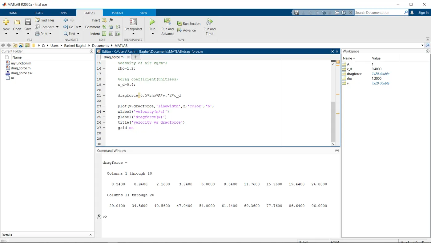
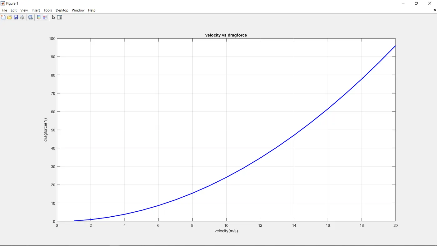
PLOT#1 Dragforce(N) varies in a PARABOLIC fashion wrt Velocity(m/s)

CODE#2

MATLAB program to plot drag coefficient vs drag force.

 
 %program to plot drag coefficient vs drag force acring on a cyclist
 
 %input variables
 
 %A= frontal area (m^2)
 A=1;
 
 %velocity (m/s);
  v=10;

  %desnity of air kg/m^3
  rho=1.2;
  
  %drag coefficient(unitless)
  c_d=[0.47 0.42 0.50 1.05 0.80];
  labels={'sphere','halfsphere','cone','cube','angled cube'}
  
  
  dragforce=0.5*rho*A*v.^2*c_d
  
  plot(c_d ,dragforce,'marker','s','markerfacecolor','r');
  text(c_d,dragforce,labels)
  xlabel('c_d')
  ylabel('dragforce(N)')
  title('drag coeff. vs dragforce')
  grid on
  

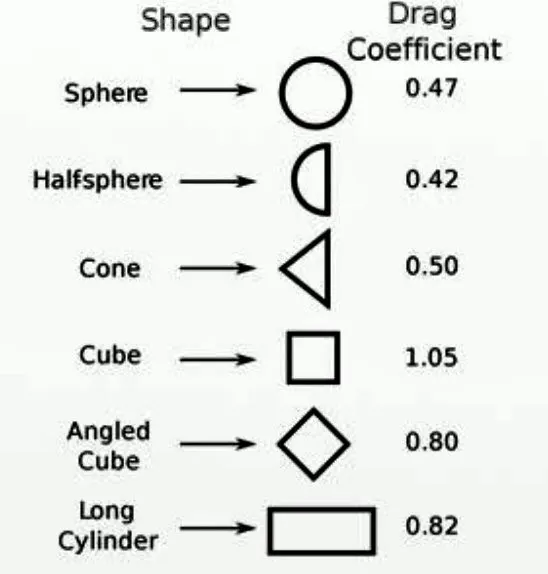
We will proceed with different values of drag coefficient corresponding to different shapes as shown below

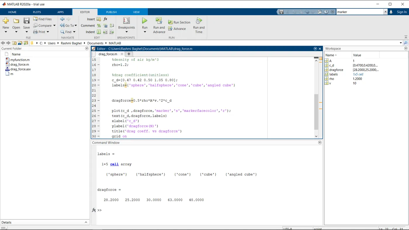
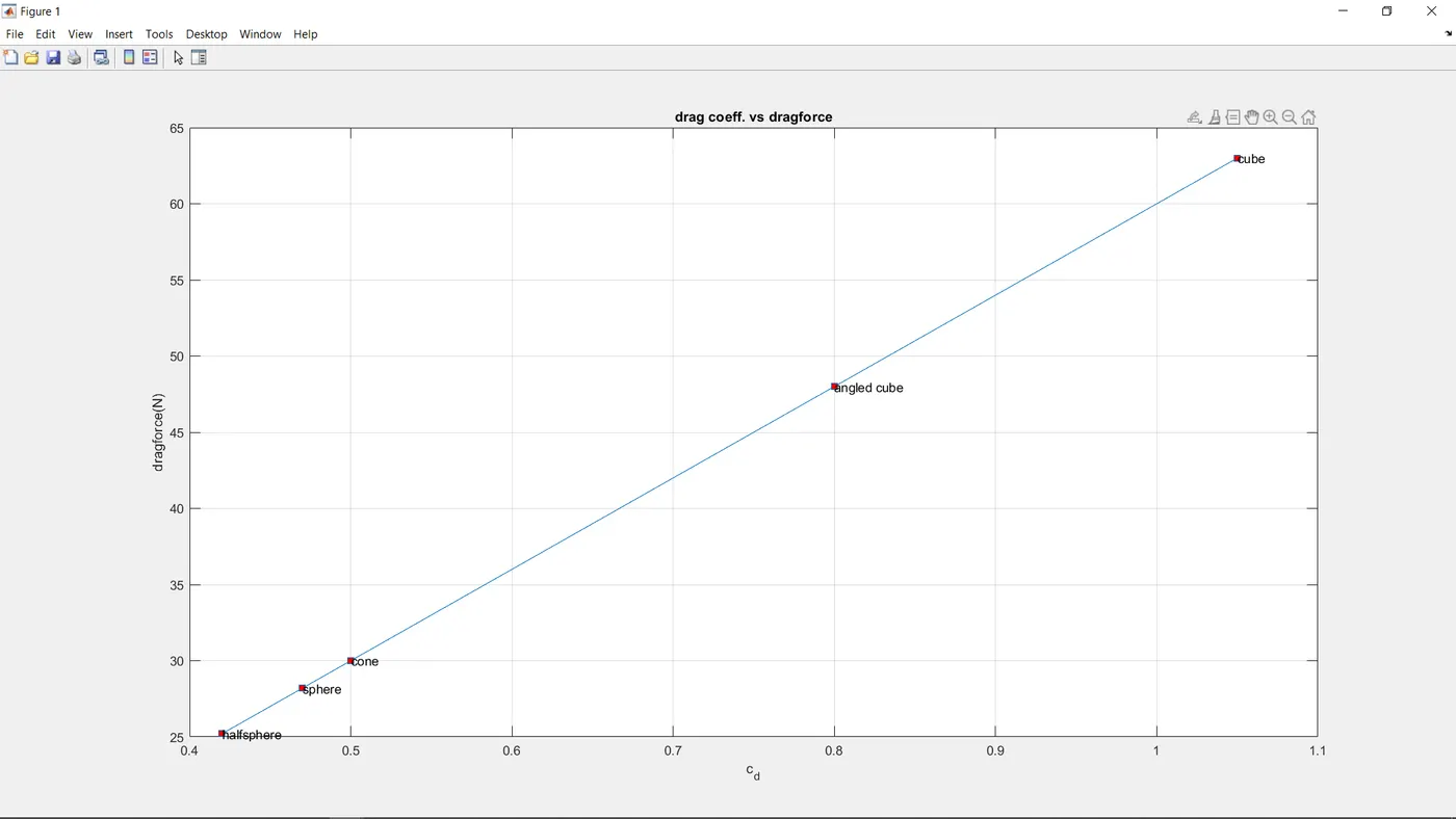
Output#2 Different values of drag force corresponding to different drag coefficients are obtained.

PLOT#3 :We can see that the drag force varies linearly with the drag coefficient(c_d_),keeping the frontal area(A) constant.

Conclusion : By looking at the above results, we can say that Dragforce is

• Directly proportional to the square of velocity.
• Directly proportional to drag coefficient.