Polynomial Curve Fit
Aim: Write a program on MATLAB to fit a linear-cubic polynomial and plot a curve fit for the ‘data’ file provided.
Objective:
1. To write code to fit a linear and cubic polynomial for the Cp data.
- To plot the linear and cubic fit curves along with the raw data points.
- To write a code to show split-wise method.
- To explain the parameters used to measure the fitness characteristics for both the curves.
- Answer the following questions
- How to make a curve fit perfectly?
- How to get the best fit?
- What could be done to improve the cubic fit?
Theory: Curve fitting is the process of constructing a curve, or mathematical function, that has the best fit to a series of data points possibly subject to constraints. Curve fitting can involve either interpolation where an exact fit to the data is required, or smoothing in which a "smooth" function is constructed that approximately fits the data
Fitting functions to data points
Most commonly, one fits a function of the form y = f(x).
Fitting lines and polynomial functions to data points
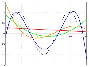
Polynomial curves fitting points generated with a sine function. The black dotted line is the "true" data, the red line is a first degree polynomial, the green line is second degree, the orange line is third degree and the blue line is fourth degree.
The first degree polynomial equation
y=ax+b
is a line with slope a. A line will connect any two points, so a first degree polynomial equation is an exact fit through any two points with distinct x coordinates.
If the order of the equation is increased to a second degree polynomial, the following results:
y=ax^2+bx+c
This will exactly fit a simple curve to three points.
If the order of the equation is increased to a third degree polynomial, the following is obtained:
y=ax^3+bx^2+cx+d
This will exactly fit four points.
The need to choose the best fit.
Goodness of fit
The goodness of fit of a statistical model describes how well it fits a set of observations. Measures of goodness of fit typically summarize the discrepancy between observed values and the values expected under the model in question.
Goodness of Fit Statistics
After using graphical methods to evaluate the goodness of fit, you should examine the goodness of fit statistics. The Curve Fitting Toolbox supports these goodness of fit statistics for parametric models:
- The sum of squares due to error (SSE)
- R-square
- Adjusted R-square
- Root mean squared error (RMSE)
-SSE is the sum of the squared differences between each observation and its group's mean. It can be used as a measure of variation within a cluster. If all cases within a cluster are identical the SSE would then be equal to 0.
The formula is: SSE=∑in(y(i)-f(x(i)))^2
-R-Square. This statistic measures how successful the fit is in explaining the variation of the data. Put another way, R-square is the square of the correlation between the response values and the predicted response values. It is also called the square of the multiple correlation coefficient and the coefficient of multiple determination.
R-square is defined as the ratio of the sum of squares of the regression (SSR) and the total sum of squares (SST). SSR is defined as
R2=SSRSST">R2=SSRSSTR2=SSRSST
where,
SSR=∑in(f(x(i))-Mean)^2
similarly,
SSE=∑in(y(i)-f(x(i)))^2
SST(sum of squared total) = SSR + SSE
-Adjusted R-squared : The adjusted R-squared is a modified version of R-squared that has been adjusted for the number of predictors in the model. The adjusted R-squared increases only if the new term improves the model more than would be expected by chance. It decreases when a predictor improves the model by less than expected by chance. The adjusted R-squared can be negative, but it’s usually not. It is always lower than the R-squared.
R^2_adj=1-[(1-R2).(n-1)/(n-k-1)]
Where, n = no. of data points
k = no. of independent variables
-Root mean square error(RMSE) : This statistic is also known as the fit standard error and the standard error of the regression
RMSE=√SSE/n
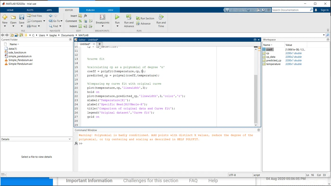
Steps to proceed with the code#1 :
1. Download the given 'data' file and make sure it exists in the same location as that of your code.
https://drive.google.com/file/d/1vWi9Vj3AdQf0gqUK1u9jwS8zg92BHGR0/view
2. Call for the provided 'data' by using the 'load' command and name the file.
3. Specify and name the parameters (here, temperature & cp) present in the 'data' file for further use.
4. We will use a 'for loop' in order to generate a polynomical of degree 'n' .
5. The 'polyfit' command is used to calculate the COEFFICIENTS of the polynomial.
6. The 'polyval' command is ussed to calculate the predicted value of 'cp'.
7. As soon as the above data is computed, plot all the curves along with their specifications using the 'plot' command.
8. Label the axes and give an appropriate title to the plot.
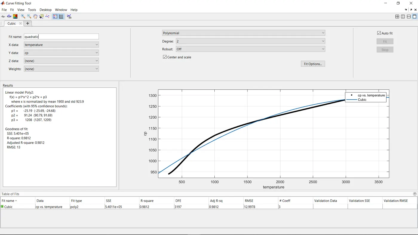
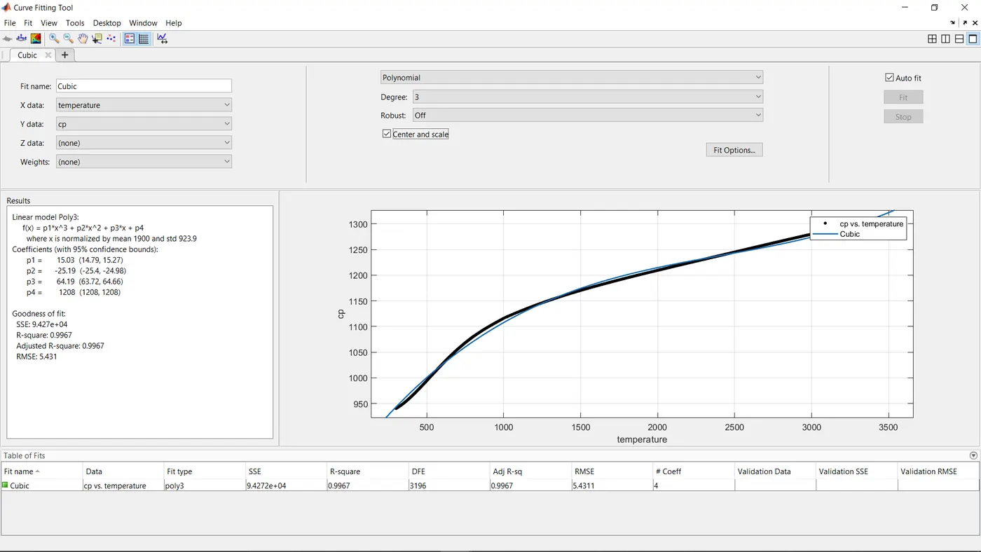
9. Use the curve fitting tool box to obtain the linear , quadratic and cubic polynomial curve fits.
code 1
clear all
close all
clc

%Curve fitting

%Loading given data
cp_data = load('data(1)');
temperature = cp_data(:,1);
cp = cp_data(:,2);


%curve fit

%calculating cp as a polynomial of degree 'n'

for i = 1:3
coeff = polyfit(temperature,cp,i);
predicted_cp(:,i) = polyval(coeff,temperature);

%Comparing my curve fit with original curve

plot(temperature,cp,'linewidth',3,'color','k');
hold on
plot(temperature,predicted_cp,'linewidth',3);
hold off
xlabel('Temperature[K]');
ylabel('Specific Heat[KJ/Kmole-K');
title('Comparison of Original data and Curve fit');
legend('Rawdata','linear','Quadratic','Cubic');

grid on
end
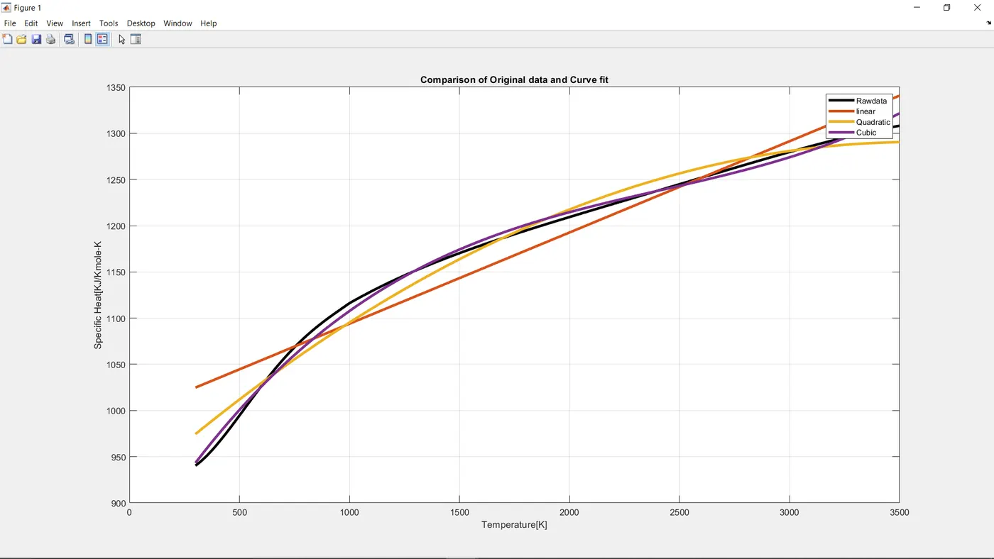
#OUTPUT : As we can see the program ran successfully .
PLOT#1: The plot shows that 'cp' is not constant and varies with Temperature.
#Outputs of the Curve Fitting Toolbox
Linear
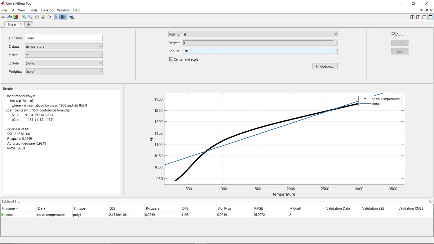
Quadratic
Cubic
Steps to proceed with the code#2:
1. Repeat the same procedure upto Step 3(code#1)
2. By using the split-wise method , segregate the the data as per your convenience.
3. Repeat steps 4,5 & 6 by computing the values of 'coefficients' and 'predicted cp' seperately for each segregation.
4. In order to minimize the dicrepancies in the curve fit , use the method of 'Goodness of fit' and specify all the parameters required along with their formulae.
5. Repeat Steps 7 & 8.
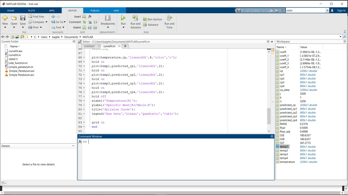
clear all
close all
clc

%Loading given data
cp_data = load('data(1)');
temperature = cp_data(:,1);
cp = cp_data(:,2);

%Splitting the data according to the range

%temperature
temp1 = cp_data(1:800,1);
temp2 = cp_data(801:1600,1);
temp3 = cp_data(1601:2400,1);
temp4 = cp_data(2401:3200,1);

%Specific Heat (Cp)
cp1 = cp_data(1:800,2);
cp2 = cp_data(801:1600,2);
cp3 = cp_data(1601:2400,2);
cp4 = cp_data(2401:3200,2);

coeff = polyfit(temperature,cp,3);
predicted_cp = polyval(coeff,temperature);

%Coefficients & predicted cp

coeff_1 = polyfit(temp1,cp1,3);
predicted_cp1 = polyval(coeff_1,temp1);

coeff_2 = polyfit(temp2,cp2,3);
predicted_cp2 = polyval(coeff_2,temp2);

coeff_3 = polyfit(temp3,cp3,3);
predicted_cp3 = polyval(coeff_3,temp3);

coeff_4 = polyfit(temp4,cp4,3);
predicted_cp4 = polyval(coeff_4,temp4);

%Goodness of fit
%Error = [y(j)-f(x(j))] | y = cp , f(x) = predicted_cp |
%Error = cp(j) - predicted_cp(j);


for j = 1:length(cp)


SSE = sum((cp(j) - predicted_cp(j)).^2);          %Sum of Squared Errors

SSR = sum((predicted_cp(j) - mean(cp(j))).^2);    %Sum of squares of regression

SST = SSR + SSE ;                                  %Sum of Squared Total

Rsqr = SSR/SST ;

% Rsqr_adj = 1 - [(1 - Rsqr)*(n-1)/(n - k - 1)]  %Adjusted R-square

n = 3200;                                        %Number of Datapoints
k = 1;                                           %Number of independent Var

Rsqr_adj = 1 - ((1 - Rsqr)*(n-1)/(n - k - 1)) ;

RMSE = sqrt(SSE/n);                              %Root mean squared error

%Plotting

plot(temperature,cp,'linewidth',5,'color','y');
hold on
plot(temp1,predicted_cp1,'linewidth',2,'linestyle','--','color','r');
plot(temp2,predicted_cp2,'linewidth',2,'color','b');
plot(temp3,predicted_cp3,'linewidth',2,'linestyle','--','color','k');
plot(temp4,predicted_cp4,'linewidth',2,'color','g');
hold off
xlabel('Temperature[K]');
ylabel('Specific Heat[KJ/Kmole-K');
title('Spliwise Curve');
legend('Raw Data','Linear','Quadratic','Cubic');

grid on
end
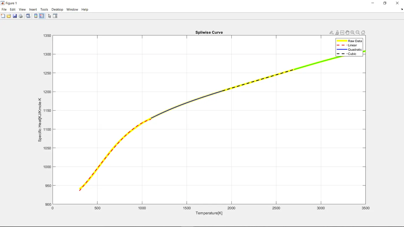
OUTPUT#2 The program was executed successfully and all the values were computed.
PLOT# 2 : As can be seen , Cp varies with temp along the segregated range
NOTE: In order to obtain a perfect curve fit, we must use the goodness of fit strategies and choose the degrees of polynomial wisely.
Coclusion : 1) The code to fit a linear/cubic polynomial was written and executed and the curve fit was obtained using the curve fitting tool box.
2) The code demonstrating the split-wise method was written and executed and the curve fit was obtained.
3) The parameters defining the goodness of fit characteristics were explained and made use of.
Reference :
https://skill-lync.com/projects/Curve-Fitting-and-criterion-to-choose-best-fit-41860