Simulation of a Simple Pendulum motion

Aim: To write a program in MATLAB for simulation of a pendulum motion.

Governing Equation: This ODE represents the equation of motion of a simple pendulum with damping.

`(d^2θ)/(dt) + b/m .(dθ)/(dt) + g/l.sin⁡θ = 0`

Where,

g = gravity in m/s^2

L = length of the pendulum in m,

m = mass of the ball in kg,

b = damping coefficient.

Theory: A simple pendulum consists of a ball (point-mass) m hanging from a (massless) string of length L and fixed at a pivot point P. When it is displaced sideways from its resting, equilibrium position, it is subject to a restoring force due to gravity that will accelerate it back toward the equilibrium position. When released, the restoring force acting on the pendulum's mass causes it to oscillate about the equilibrium position, swinging it back and forth.

The time it takes to complete one oscillation is known as its Time Period(T)

The number of oscillations that occur per unit time and is inverse of the period(T), is known as the frequency of the oscillations f = 1/T

The maximum displacement of the mass from its equilibrium position is known as the amplitude of the oscillations.

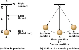
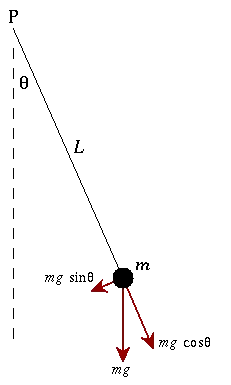
Objective: 1) To simulate the motion of a Simple Pendulum using MATLAB.

2) To create an animation file of the above.

Solution:

Coding Language: MATLAB

Code #1

%2nd order differential equation

%inputs

b= 0.05;   % damping coefficient 
g= 9.81;   % acceleration due to gravity(m/s^2)
l= 1;      % length of rope(m)
m= 1;      % mass (kg)


%initial condition
theta_0 = [0;3];

%time
t_span=linspace(0,15,400);

%ODE
[t,R]= ode45(@(t,theta)ode_function(t,theta,b,g,l,m),t_span,theta_0);

%plot 1
figure(1)
plot(t,R(:,1));
hold on
plot(t,R(:,2));
hold off
xlabel('Time(sec)')
ylabel('Angular Displacement(rad) & Angular Velocity(rad/sec)')
legend('Angular Disp','Angular vel')
grid on

ct=1;
for i=1:length(t_span)
    theta_3 = R(i,1);
    
    x0=0; 
    y0=0;
    
    x1=l*sin(theta_3);
    y1=-l*cos(theta_3);
    
    %plot 2
    figure (2)
    
    plot([-0.5,0.5],[0,0],'linewidth',3,'color','r')
    hold on
    plot([0,0],[0,-1],'linewidth',1,'linestyle','--')
    plot([x0 x1],[y0 y1],'linewidth',2,'color','b')
    plot(x1,y1,'marker','o','markersize',10,'markerfacecolor','y')
    
    hold off
    xlabel('X Axis')
    ylabel('y Axis')
    title('Transient Behavior of a Simple Pendulum')
    grid on
    axis([-1.5 1.5 -1.2 1])
    pause(0.03)
    
    M(ct)=getframe(gcf);
    ct=ct+1;
end

%Animation
 movie(M);
 videofile=VideoWriter('Simple_Pendulum.avi','Uncompressed AVI');
 open(videofile);
 writeVideo(videofile,M);
 close(videofile);

Function: The function [dtheta_dt] needs to be called in order to solve the above program.

Solving the ODE

`(d^2 θ)/(dt^2) + b/m.(dθ)/(dt) + g/l.sin⁡θ = 0` .....(1)

let `θ= θ1`

then,

`(d^2θ1)/(dt^2) + b/m.(dθ1)/(dt) + g/l.sin⁡θ1 = 0`

let `(dθ)/dt = (dθ1)/dt = θ2` .....(2)

putting in (1), we get

`(dθ2)/(dt) + b/m .θ2 + g/l.sin⁡θ1 = 0`

`(dθ2)/(dt) = - (b/m) .θ2 - (g/l).sin⁡θ1` .....(3)

function[dtheta_dt]= ode_function(t,theta, b,g,l,m)
    theta1 = theta(1);
    theta2 = theta(2);
    dtheta1_dt = theta2;
    dtheta2_dt = -(b/m)*theta2 - (g/l)*sin(theta1);
    dtheta_dt = [dtheta1_dt ; dtheta2_dt];
end

Output: As we can see, the program was executed successfully.

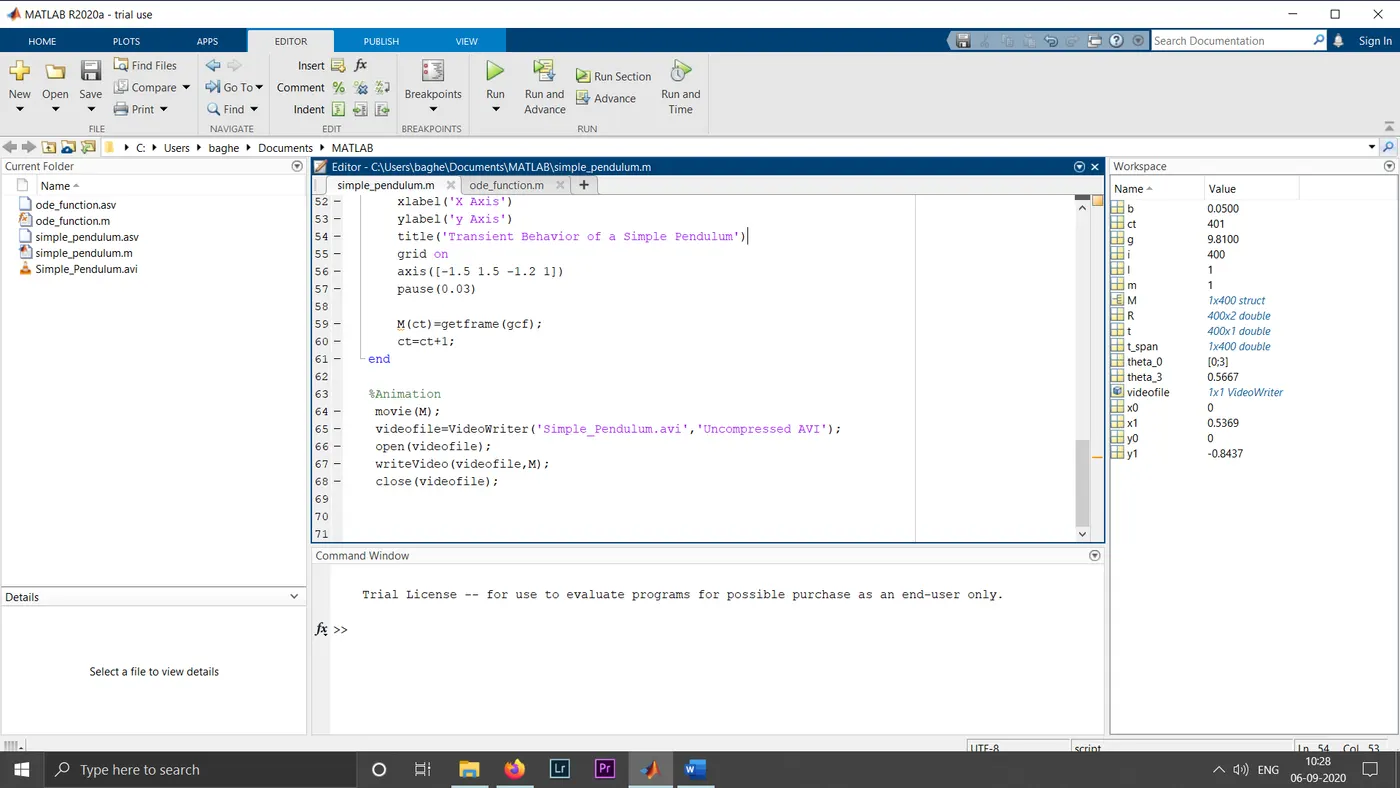
Plot : The plot shows the rate of change of angular disp(blue) and angular velocity(red).

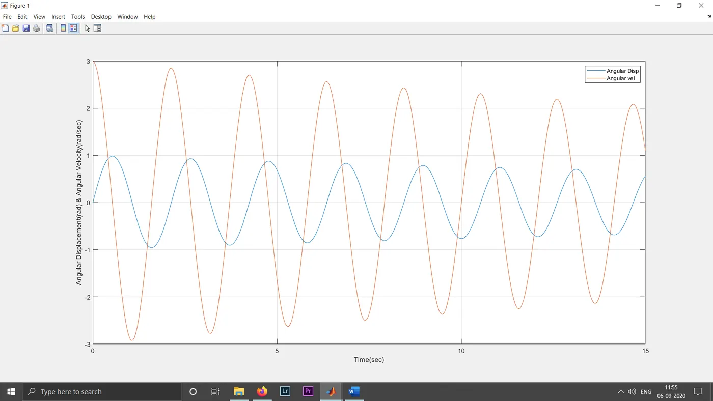
Animation File

https://drive.google.com/drive/folders/1d888otRre2LK9736Pm90RUxvSvxtaSd5?usp=sharing

Conclusion: The MATLAB program was executed successfully and the animation of pendulum motion was obtained.