Solving an Otto cycle and determining its efficiency using MATLAB
Aim: To solve an Otto Cycle and make plots using MATLAB.
Governing Equations:
PVγ=constant
PV/T=constant
VS=π4.d2.L
Vc=Vscr−1
cr=V2V1=V3V4
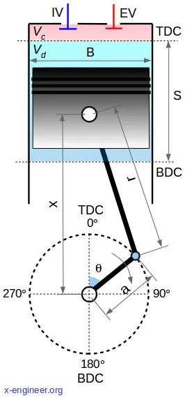
Vθ=[1+12(cr−1)√(1+R−cosθ−√(R2−sinθ2))].Vc
ηo=1−T4−T1T3−T2=1−1crγ−1
Where,
P = pressure(Pa)
V = volume(m^3)
T = temperature(K)
γ=isentropic.index">γ=isentropic.index
cr=compressionratio
Vc
=clearance volume
Vs
= swept volum`
θ
= crank angle
ηo
= otto cycle efficiency
THEORY:
An Otto Cycle is an idealized thermodynamic cycle that describes the functioning of a typical spark ignition combustion engine. It is the thermodynamic cycle most commonly found in automobile engines.The Otto cycle is a description of what happens to a mass of gas as it is subjected to changes of pressure, temperature, volume, addition of heat, and removal of heat. The mass of gas that is subjected to those changes is called the system. The system, in this case, is defined to be the fluid (gas) within the cylinder. By describing the changes that take place within the system, it will also describe in inverse, the system's effect on the environment. In the case of the Otto cycle, the effect will be to produce enough net work from the system so as to propel an automobile and its occupants in the environment.
The Otto cycle is constructed from:
1)Top and bottom of the loop: a pair of quasi-parallel and isentropic processes (frictionless, adiabatic reversible).
2)Left and right sides of the loop: a pair of parallel isochoric process (constant volume).
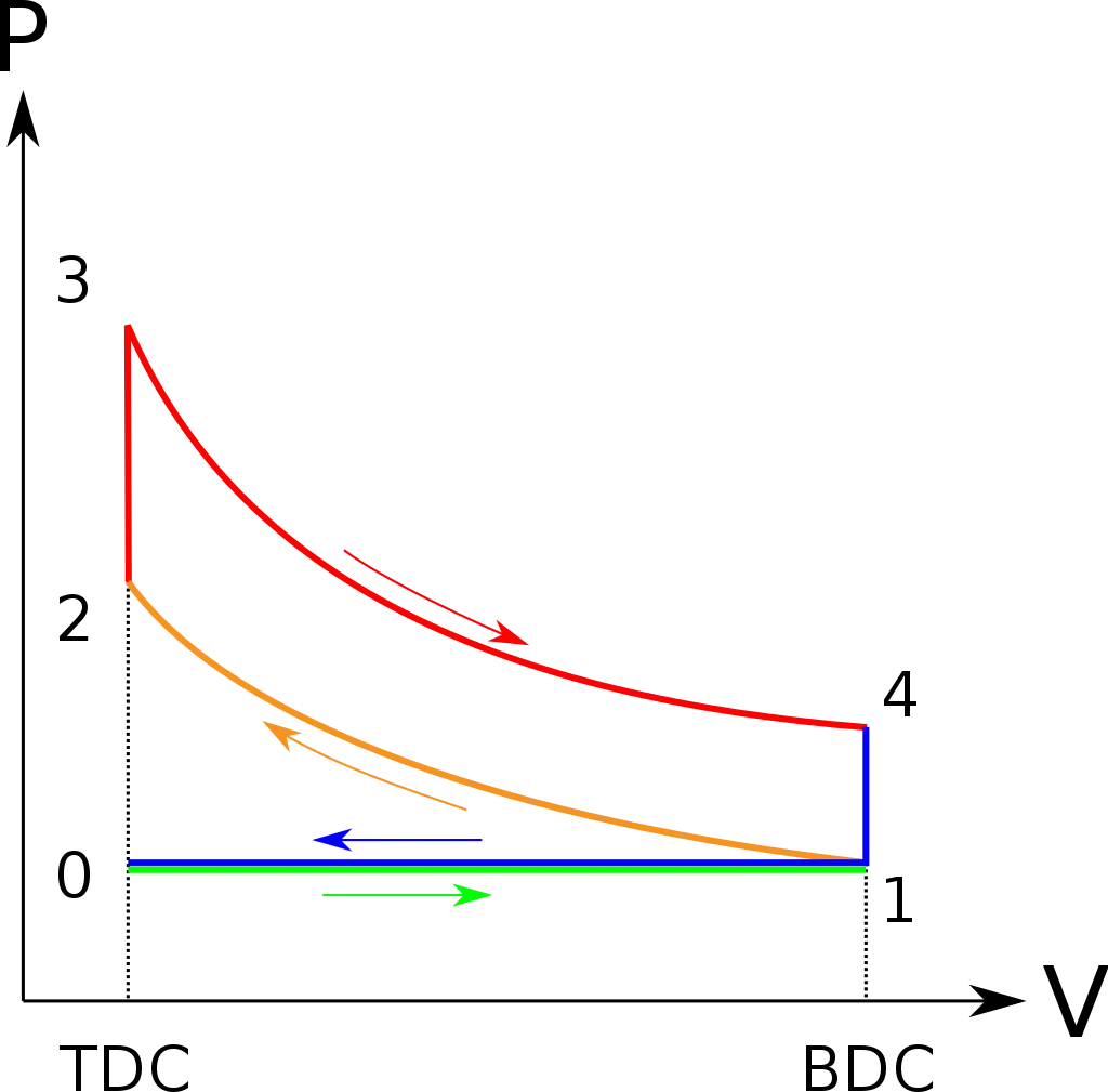
Process 0–1 intake stroke
A mass of air (working fluid) is drawn into the cylinder, from 0 to 1, at atmospheric pressure (constant pressure) through the open intake valve, while the exhaust valve is closed during this process. The intake valve closes at point 1.
Process 1–2 compression stroke (B on diagrams)
Piston moves from crank end (BDC, bottom dead centre and maximum volume) to cylinder head end (TDC, top dead centre and minimum volume) as the working gas with initial state 1 is compressed isentropically to state point 2, through compression ratio (V1/V2).
Process 2–3 ignition phase
The piston is momentarily at rest at TDC. During this instant, which is known as the ignition phase, the air/fuel mixture remains in a small volume at the top of the compression stroke. Heat is added to the working fluid by the combustion of the injected fuel, with the volume essentially being held constant.
Process 3–4 expansion stroke
The increased high pressure exerts a force on the piston and pushes it towards the BDC. Expansion of working fluid takes place isentropically and work is done by the system on the piston. The volume ratio {displaystyle V_{4}/V_{3}}V4/DSFKSDis called the "isentropic expansion ratio". (For the Otto cycle is the same as the compression ratio {displaystyle V_{1}/V_{2}}VMechanically this is the expansion of the hot gaseous mixture in the cylinder known as expansion (power) stroke.
Process 4–1 idealized heat rejection
The piston is momentarily at rest at BDC.The working gas pressure drops instantaneously from point 4 to point 1 during a constant volume process as heat is removed to an idealized external sink that is brought into contact with the cylinder head. In modern internal combustion engines, the heat-sink may be surrounding air (for low powered engines), or a circulating fluid, such as coolant. The gas has returned to state 1.
Process 1-0 exhaust stroke
The exhaust valve opens at point 1.As the piston moves from "BDC" (point 1) to "TDC" (point 0) with the exhaust valve opened, the gaseous mixture is vented to the atmosphere and the process starts anew.
Piston Kinematics of an Internal Combustion Engine:
Automotive industry deals with reciprocating engines, in which the piston has a linear motion within the cylinder. The crank mechanism transforms the linear movement of the piston into rotational movement of the crankshaft.Because of this kind of movement, the piston’s velocity goes through zero at the top dead centre(TDC) and bottom dead centre (BDC) positions.
Objectives
- Solve and plot P-V diagram of an Otto Cycle.
- To study piston Kinematics of an Otto Cycle.
- To calculate and plot the thermal efficiency.
Language Used; MATLAB
Solution;
By using the above governing equations and the given variables, the otto cycle has been solved.
CODE#1 Program to plot P-V dia of an Otto CYCLE
%Program to solve  an Otto cycle using MATLAB and make plots

%Engine geometric parameters

%bore
d=0.2;
%sroke
L=0.3;
%connecting rod length
c_d=0.25;
%compression ratio
r_c=12;

%input state variables

% p, t, v represent pressures(bar) , temperature(K) and volume at different states
t3=3000; %input

%state variables at state point 1
p1=101325;
t1=600;
gamma=1.4;

%swept and clearance volume
v_swept=pi/4*d^2*L;
v_clearance= v_swept/(r_c-1);

v1=v_swept + v_clearance;
v2=v_clearance;


%state variables at state point 2

% For an isentropic process, pv^gamma=constant
%p1v1^gamma=p2v2^gamma|%p2=p1*(v1/v2)^gamma = p1*r_c^gamma
p2= p1*r_c^gamma;

%To compute t2, we will use the ideal gas equation pv/t =constant
%p1v1/t1=p2v2/t2 | t2= p2*v2*t1/(p1*v1)
t2= p2*v2*t1/(p1*v1);

constant_c=p1*v1^gamma;
V_compression=engine_kinematics(d,L,c_d,r_c,180,0);
P_compression=constant_c./V_compression.^gamma;


%state variables at state point 3 (constant volume combustion)
 v3=v2;

 %%p3v3/t3=p2v2/t2 |%p3=p2*t3/t2
 p3=p2*t3/t2;

 constant_c=p3*v3^gamma;
 V_expansion=engine_kinematics(d,L,c_d,r_c,0,180);
 P_expansion=constant_c./V_expansion.^gamma;

%state variables at state point 4
 v4=v1;

%p3v3^gamma=p4v4^gamma | p4=p3*(v3/v4)^gamma
p4=p3*(v3/v4)^gamma;
%p3*v3/t3=p4*v4/t4
t4=(p4*v4*t3)/(p3*v3);

%Efficiency
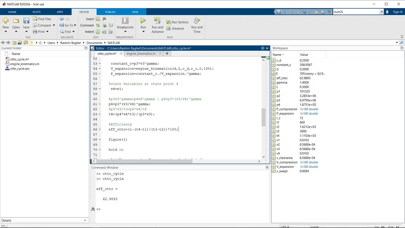
eff_otto=(1-(t4-t1)/(t3-t2))*100;

figure(1)

hold on

plot(V_compression,P_compression,'color','r')
plot([v2 v3],[p2 p3],'g')
plot(V_expansion,P_expansion,'color','y')
plot([v1 v4],[p1 p4],'color','k')
plot(v1,p1,'*','color','b')
plot(v2,p2,'*','color','b')
plot(v3,p3,'*','color','b')
plot(v4,p4,'*','color','b')
text(v1,p1,'1')
text(v2,p2,'2')
text(v3,p3,'3')
text(v4,p4,'4')

xlabel('Volume (m^3)')
ylabel('Pressure (Pa)')
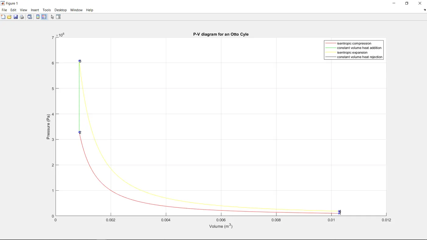
title('P-V diagram for an Otto Cyle')
legend('isentropic compression','constant volume heat addition','isentropic expansion','constant volume heat rejection')
grid onOUTPUT#1 As we can see, the P-V plot is obtained based on the inputs provided.
-Otto cycle efficiency has been calculated
CODE#2 The following function was used to obtain the actual volume (wrt the crank angle)
function[V]=engine_kinematics(d,L,c_d,r_c,start_crank,end_crank)

a=L/2;
R=c_d/a;
v_swept=pi/4*d^2*L;
v_clearance=v_swept/(r_c-1) ;

theta=linspace(start_crank,end_crank,180);

term1=0.5*(r_c-1);
term2=R+1-cosd(theta) ;

term3=(R^2-sind(theta).^2).^0.5;

V=(1+term1*(term2-term3)).*v_clearance ;
plot(v)
xlabel('crank angle(degree)')
ylabel('volume(m^3)')
end
CONCLUSION:
Based on the results obtained, we can say that the objective (to solve an otto cycle and plot the P-V diagram) has been fulfilled.
ηo=62.9%">ηo=62.9%