Parsing NASA's thermodynamic data

AIM: To parse NASA’s Thermodynamic data and perform the given tasks using MATLAB.

FORMULAE:

Where a1, a2, a3, a4, a5, a6, a7 are local high-temperature coefficients

A1, A2, A3, A4, A5, A6, A7 are local low-temperature coefficients

Cp = specific Heat (j/mole K)

S = Entropy (J/K)

H = enthalpy (J)

R = Universal Gas constant ( J/mole K)

OBJECTIVE:

1. To write a program to extract 14 coefficients from all the species and calculate the Specific Heat (Cp), Enthalpy(H) & Entropy(S) for each of them.
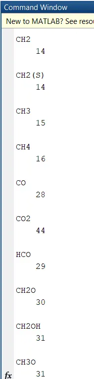
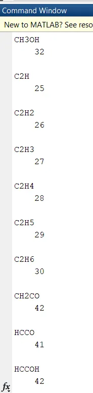
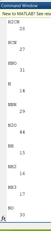
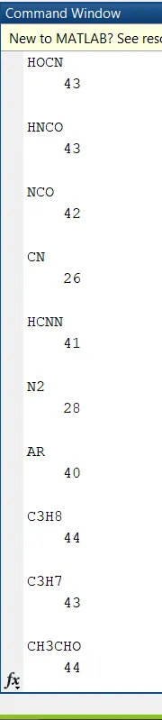
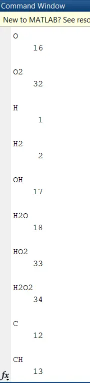
2. To calculate the molecular weight of all the species and display it on the command window.
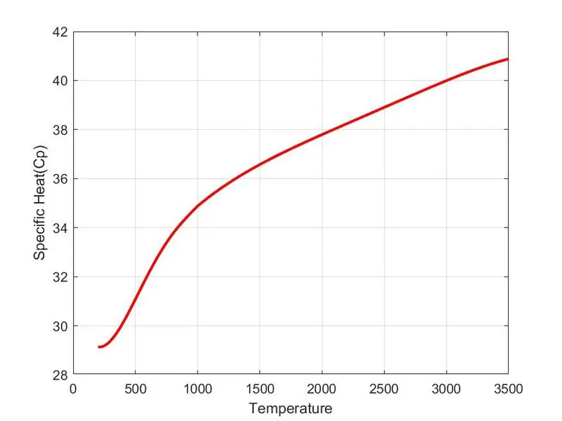
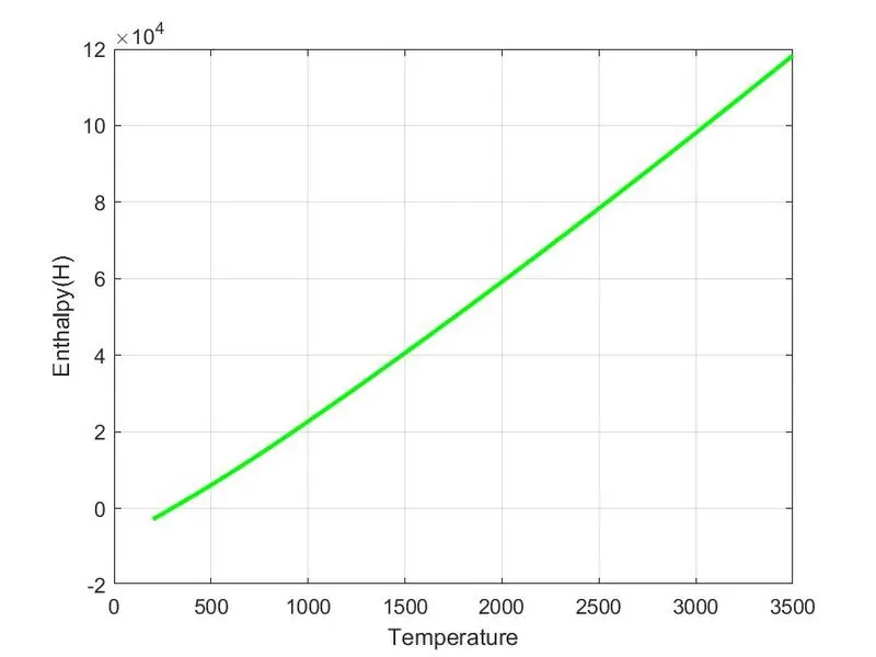
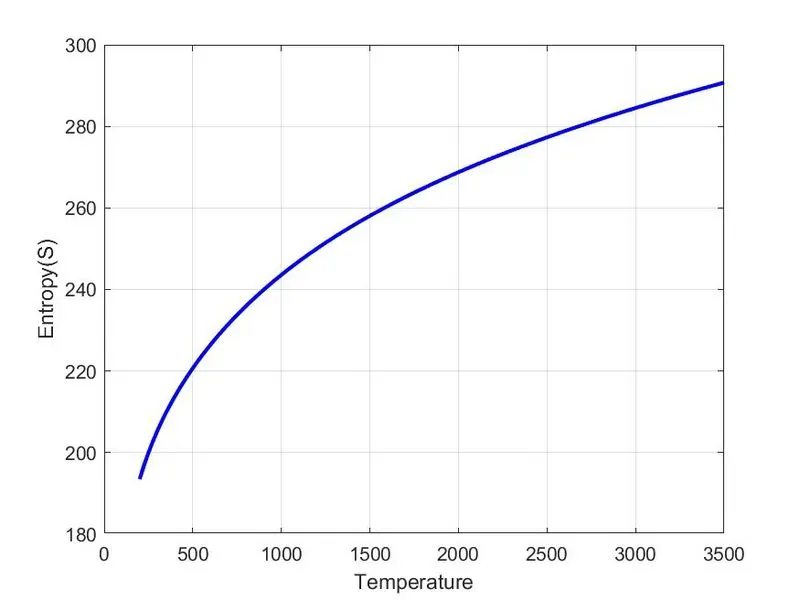
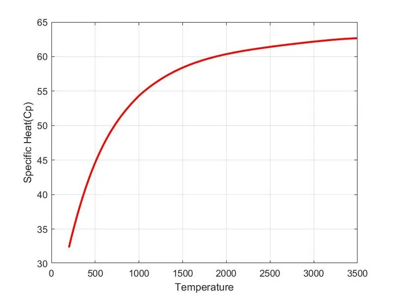
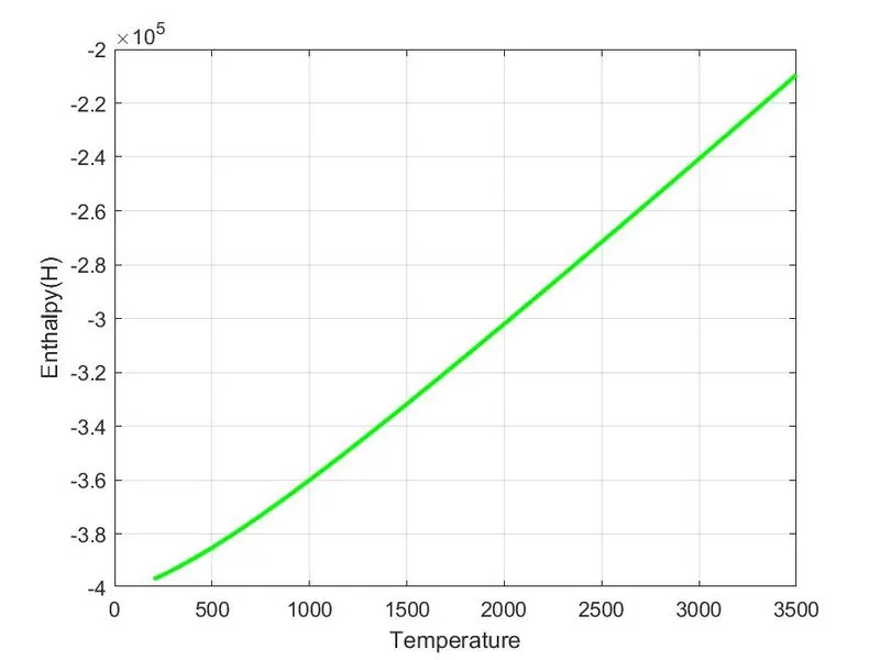
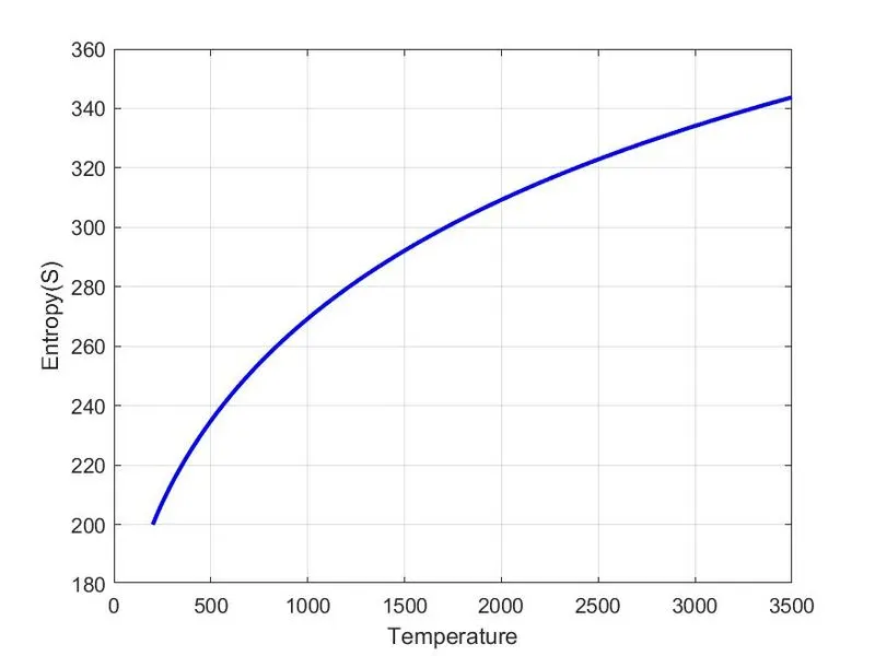
3. Plot Cp, H, and S for the species at ‘local temperature’.
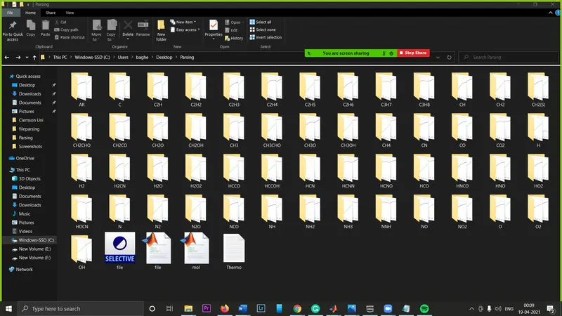
4. To create a directory and save images of each plot in the respective element folder.

THEORY:

Parsing in computer languages refers to the syntactic analysis of the input code into its components parts in order to facilitate the writing of compilers and interpreters. It can be used to describe split or separation. Parsing a file means reading in a data stream of some sort and building an in-memory model of the semantic content of that data. This aims at facilitating performing some kind of transformation on the data.

PROCEDURE:

1. Open the given data file using ‘fopen’ command and read the data using ‘r’.
2. Use ‘fgetl’ command to read the data linewise and convert it into a string array.
3. Use ‘strsplit’ to remove the unwanted space in between characters. Define the global temperatures and convert them into numbers using ‘str2num’ or ‘str2double’.
4. Keep a check on the variable values in the workspace.
5. For extracting the species data, we need to find the no. of species first.

• Use ‘while’ loop and ‘strfind’ command to search for the last character (‘END’ in this case) of the data file.
• It will give the line number to which this character belongs. Since we’ve already defined the first set of lines, we’ll subtract those lines from the total number of lines(c).
• Each species’ data is distributed in 4 lines so, (c-6)/4 will give us the total number of species/elements.

6. Use the ‘for’ loop as we need to perform the same set of operations for every species.

• First, define and read the characters line by line according to their positions.
• Omit the first five lines and declare ‘L1’, which contains the element, as our first line.
• Create an array for each character occupying different positions and convert it into numbers.
• Find the position of ‘E’ and then locate each of the coefficients for low as well as high local temperature ranges.
• Create four such lines and follow the same procedure.

7. Once, the coefficients are extracted, calculate Cp, H and S.
8. Obtain the required plots.
9. Create a directory using ‘mkdir’ command where the obtained plots can be saved (as images) in their respective element folder.
10. Write a function to calculate the molecular weight of the species and call the function in the main program.
11. Display the weights in the command window using ‘disp’ command.
12. Put an ‘End’ to the loop.

MATLAB PROGRAM:

% Parsing NASA's thermodynamic data
f1 = fopen('Thermo.txt','r');  % Reading data from the file

%Defining the first set of lines
Header = fgetl(f1); %header
global_temp_array=fgetl(f1); 
fgetl(f1);
fgetl(f1);
fgetl(f1);

%Global temperature range
gtemp_range = strsplit(global_temp_array,' ');
global_low_temp = str2double(gtemp_range{2});
global_mid_temp = str2double(gtemp_range{3});
global_high_temp = str2double(gtemp_range{4});

%Extracting species data
%To find the no. of species
c = 0;
while 1
    line = fgetl(f1);
    c = c+1;
    compare = strfind(line,'END');
    if compare == 1
        break
    else
        continue
    end
end

no_species = (c-6)/4;

%High temp coefficients= a1, a2, a3, a4, a5, a6, a7
%Low temp coefficients = A1, A2, A3, A4, A5, A6, A7

for i= 1:53
     L1=fgetl(f1);
     char = strsplit(L1);
element_name = char{1};

 %local temperature range
 G_pos = strfind(L1,'G');    %Locating 'G' to obtain local temperatures
 temp = L1(G_pos+3:end);
 local_temp = strsplit(temp);
 llow_temp = str2double(local_temp{2});
 lmid_temp = str2double(local_temp{4});
 lhigh_temp = str2double(local_temp{3});
 
 L2=fgetl(f1);
 E_pos1 = strfind(L2,'E');   %Locating 'E' to obtain position of coeff==
 
 %Extracting coefficients
 a1 = str2double(L2(1:E_pos1(1)+3));
 a2 = str2double(L2(E_pos1(1)+4:E_pos1(2)+3));
 a3 = str2double(L2(E_pos1(2)+4:E_pos1(3)+3));
 a4 = str2double(L2(E_pos1(3)+4:E_pos1(4)+3));
 a5 = str2double(L2(E_pos1(4)+4:E_pos1(5)+3));
 
 L3=fgetl(f1);
 E_pos2 = strfind(L3,'E');
 a6 = str2double(L3(1:E_pos2(1)+3));
 a7 = str2double(L3(E_pos2(1)+4:E_pos2(2)+3));
 A1 = str2double(L3(E_pos2(2)+4:E_pos2(3)+3));
 A2 = str2double(L3(E_pos2(3)+4:E_pos2(4)+3));
 A3 = str2double(L3(E_pos2(4)+4:E_pos2(5)+3));
 
 L4=fgetl(f1);
 E_pos3 = strfind(L4,'E');
 A4 = str2double(L4(1:E_pos3(1)+3));
 A5 = str2double(L4(E_pos3(1)+4:E_pos3(2)+3));
 A6 = str2double(L4(E_pos3(2)+4:E_pos3(3)+3));
 A7 = str2double(L4(E_pos3(3)+4:E_pos3(4)+3));
 
 %Declaring temperature range for plotting the graph
 t_range = linspace(llow_temp,lhigh_temp,200);
 t= t_range;
 R=8.314;
Cp = zeros(size(t));
H = zeros(size(t));
S = zeros(size(t));

 for j = 1:length(t)
     if t(j) > lmid_temp
     
 Cp(j)= (a1 + a2*t(j) + a3*t(j).^2 + a4*t(j).^3 + a5*t(j).^4)*R ;
 H(j)= (a1 + a2*(t(j)/2) + a3*((t(j).^2)/3)+ a4*((t(j).^3)/4) + a5*((t(j).^4)/5) + a6/t(j))*R*t(j);
 S(j) = R*(a1*log(t(j)) + a2*t(j) + a3*(t(j).^2)/2 + a4*(t(j).^3)/3 + a5*(t(j).^4)/4 + a7);
 
     else
         
 Cp(j) = R*(A1 + A2*t(j) + A3*t(j).^2 + A4*t(j).^3 + A5*t(j).^4);
 H(j)= (A1 + A2*(t(j)/2) + A3*((t(j).^2)/3)+ A4*((t(j).^3)/4) + A5*((t(j).^4)/5) + A6/t(j))*R*t(j);
 S(j) = R*(A1*log(t(j)) + A2*t(j) + A3*(t(j).^2)/2 + A4*(t(j).^3)/3 + A5*(t(j).^4)/4 + A7);
         
     end
 end
 
 %Obtaining the plots
 figure(1)
 plot(t,Cp,'linewidth',2,'color','r');
 xlabel('Temperature');
 ylabel('Specific Heat(Cp)');
 grid on
 
 figure(2)
 plot(t,H,'linewidth',2,'color','g');
 xlabel('Temperature');
 ylabel('Enthalpy(H)');
 grid on
 
 figure(3)
 plot(t,S,'linewidth',2,'color','b');
 xlabel('Temperature');
 ylabel('Entropy(S)');
 grid on
 
 loc_program =(['C:UsersbagheDesktopParsing']);  %Specifying the location of the prog
 mkdir("C:UsersbagheDesktopParsing",element_name); % Creating a directory
 cd(element_name)
 saveas(1,'Cp vs t','jpg')    % saving the plots as images
 saveas(2,'H vs t','jpg')
 saveas(3,'S vs t','jpg')
 cd(loc_program)
 
 molecular_weight = mol(element_name);    % calling out the function for obtaining molecular weight
end

Function to obtain the Molecular weight of the species

function[wt]= mol(element_name)
Atom = ['H','C' ,'N','O', 'A'];
atomic_weight = [1,12,14,16,40];
wt = 0;
for k = 1:length(element_name)
    for l = 1:length(Atom)
tf = strcmp(element_name(k),Atom(l));
if tf == 1
    wt = wt + atomic_weight(l);
    x = l;
end
    end
%Convwerting string to number    
index = str2double(element_name(k));
if index > 1
    wt = wt + atomic_weight(x)*(index-1);
end
end

disp(element_name)
disp(wt)
end

Screenshots displaying molecular weights in the command window.

Plots :

O2

N2

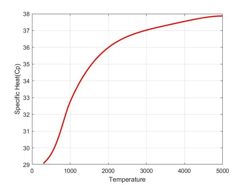
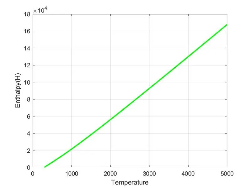
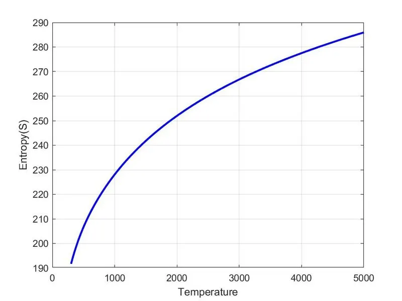
CO2

SCREENSHOT of the folders containing plots.

CONCLUSION: NASA's thermodynamic data has been parsed successfully and the required tasks have been performed.