Aim:

• Write code in MATLAB to fit a linear and cubic polynomial for the Cp data.
• Plot the linear and cubic fit curves along with the raw data points. Title and axes labels are a must, legends could be shown if necessary.
• Write a code to show split-wise method.
• Explain the parameters used to measure the fitness characteristics for both the curves.

Note: You could use the Curve fitting toolbox in MATLAB to validate your fitness characteristics. (This is optional)

Background:

Curve fitting is a process of constructing a curve or mathematical functions, which possess the closest proximity to the real series of data.

Curve fitting can involve either interpolation, where an exact fit to the data is required, or smoothing, in which a "smooth" function is constructed that approximately fits the data.

Extrapolation refers to the use of a fitted curve beyond the range of the observed data, and is subject to a degree of uncertainty since it may reflect the method used to construct the curve as much as it reflects the observed data.

Fitting lines and polynomial functions to data points:

The first-degree polynomial equation

is a line with slope a. A line will connect any two points, so a first-degree polynomial equation is an exact fit through any two points with distinct x coordinates.

If the order of the equation is increased to a second-degree polynomial, the following results:

This will exactly fit a simple curve to three points.

If the order of the equation is increased to a third-degree polynomial, the following is obtained:

This will exactly fit four points.

A more general statement would be to say it will exactly fit four constraints. Each constraint can be a point, angle, or curvature.

Programme Code:

close all
clear all
clc
 
% Loading 'data file'. 
 
cp_data = load('data');
 
% Assigning names to both the columns in data file.
 
temperature = cp_data(:,1);
cp = cp_data(:,2);
 
% Curve fit
 
co_effs1 = polyfit(temperature,cp,1);
predicted_cp1 = polyval(co_effs1,temperature);
 
co_effs2 = polyfit(temperature,cp,3);
predicted_cp2 = polyval(co_effs2,temperature);
 
% Plotting and comparing the curve fit with the original data
 
plot (temperature, cp, 'linewidth',2, 'color','k');
xlabel('Temperature [K]');
ylabel('Specific heat [kJ / kmol-K]');
title('Specific heat of oxygen vs Temperature')
hold on
 
plot(temperature,predicted_cp1, 'linewidth',2, 'color','m')
plot(temperature,predicted_cp2, 'linewidth',2, 'color','g')
 
legend('original dataset','linear curve fit','cubic curve fit')
 
% Calculating errors using RMSE and R-square for Linear and Cubic fit.
 
% RMS
n = length(temperature);
RMSE1 = sqrt (sum(abs(predicted_cp1 - cp).^2) / n)
RMSE2 = sqrt (sum(abs(predicted_cp2 - cp).^2) / n)
 
% R-square
n1 = length (cp);
Avg_cp = sum(cp)/n1 ;
SSres1 = sum((cp - predicted_cp1).^2);
SSres2 = sum((cp - predicted_cp2).^2);
SStot = sum((cp - Avg_cp).^2);
 
R_square1 = 1 - (SSres1/SStot)
R_square2 = 1 - (SSres2/SStot)
 

Programme Code with comments:

close all

clear all

clc

% Loading 'data file'.

% Make sure that the data file is in same directory as Programme code file.

cp_data = load('data');

% Assigning names to both the columns in data file.

% Here, cp(Specific Heat) is a dependent variable.

temperature = cp_data(:,1);

cp = cp_data(:,2);

% Curve fit

% "polyfit" command helps in finding Polynomial coefficients to aid in predicting cp values.

% "polyval" command uses Polynomial coefficients and independent variables to predict dependent variables.

% eg. cp = a*T^2 + b*T^2 + c, where a,b & c are coefficients.

% co_effs1 are the coefficient for degree one/linear polynomial.

% co_effs2 are the coefficient for degree two/cubic polynomial.

co_effs1 = polyfit(temperature,cp,1);

predicted_cp1 = polyval(co_effs1,temperature);

co_effs2 = polyfit(temperature,cp,3);

predicted_cp2 = polyval(co_effs2,temperature);

% Plotting and comparing the curve fit with the original data

plot (temperature, cp, 'linewidth',2, 'color','k');

xlabel('Temperature [K]');

ylabel('Specific heat [kJ / kmol-K]');

title('Specific heat of oxygen vs Temperature')

hold on

plot(temperature,predicted_cp1, 'linewidth',2, 'color','m')

plot(temperature,predicted_cp2, 'linewidth',2, 'color','g')

legend('original dataset','linear curve fit','cubic curve fit')

% Calculating errors using RMSE and R-square for Linear and Cubic fit.

% Note:-

% Y = abs( X ) returns the absolute value of each element in array X .

% If X is complex, abs(X) returns the complex magnitude.

% RMS

n = length(temperature);

RMSE1 = sqrt (sum(abs(predicted_cp1 - cp).^2) / n)

RMSE2 = sqrt (sum(abs(predicted_cp2 - cp).^2) / n)

% R-square

n1 = length (cp);

Avg_cp = sum(cp)/n1 ;

SSres1 = sum((cp - predicted_cp1).^2);

SSres2 = sum((cp - predicted_cp2).^2);

SStot = sum((cp - Avg_cp).^2);

R_square1 = 1 - (SSres1/SStot)

R_square2 = 1 - (SSres2/SStot)

Plot:

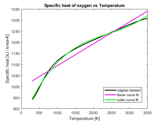
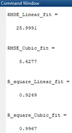
Observation:

As seen from the Plot, the cubic polynomial fit has more accurate fit than the linear polynomial fit.

The RMSE error value for Linear Poly-fit is more than the Cubic Poly-fit. And R-Square value for Cubic is more than linear fit. And we know that, Lower the RMSE or Higher the R-square, more accurate is our curve fit or predicted value. So, we can conclude by saying, lower degree polynomial functions have more deviation than the higher degree polynomial functions, this is essentially true when our data plot is non-linear.

Code for Split-wise Method with comments:

In split-wise method we will divide our data set of temperature and cp into 4 equal parts. Then we will apply the Polynomial fit separately to all 4 data set.

In the following code we will Split the entire data into 4 equal sets (for temperature and cp). Then to all 4 data set we will apply Curve fit using polynomial function of second degree. Finally, we will compare the Curve fit of combined data set and split-wise data set for second degree polynomial fit, by using the plot.

close all
clear all
clc
 
% Loading data file.
 
cp_data = load('data');
 
% Assigning names to both the columns in data file.
 
temperature = cp_data(:,1);
cp = cp_data(:,2);
 
% Curve fit using 2 degree polynomial.
 
co_effs = polyfit(temperature,cp,2);
predicted_cp = polyval(co_effs,temperature);
 
 
% Curve fitting using SplitWise polyjnomial of second degree. 
% Spliting data in 4 groups.
 
temperature1 = temperature(1:800, 1);
cp1 = cp(1:800,1);
 
temperature2 = temperature(801:1600, 1);
cp2 = cp(801:1600, 1);
 
temperature3 = temperature(1601:2400, 1);
cp3 = cp(1601:2400, 1);
 
temperature4 = temperature(2401:3200, 1);
cp4 = cp(2401:3200, 1);
 
co_effs1 = polyfit(temperature1,cp1,2);
predicted_cp1 = polyval(co_effs1,temperature1);
 
co_effs2 = polyfit(temperature2,cp2,2);
predicted_cp2 = polyval(co_effs2, temperature2);
 
co_effs3 = polyfit(temperature3,cp3,2);
predicted_cp3 = polyval(co_effs3, temperature3);
 
co_effs4 = polyfit(temperature4,cp4,2);
predicted_cp4 = polyval(co_effs4,temperature4);
 
% Plotting and comparing the curve fit with the original data
 
plot (temperature, cp, 'linewidth',4, 'color','k');
xlabel('Temperature [K]');
ylabel('Specific heat [kJ / kmol-K]');
title('Specific heat of oxygen vs Temperature')
 
hold on
 
plot (temperature, predicted_cp, 'k--')
 
plot(temperature1,predicted_cp1, 'linewidth',2, 'color','m')
plot(temperature2,predicted_cp2, 'linewidth',2, 'color','g')
plot(temperature3,predicted_cp3, 'linewidth',2, 'color','b')
plot(temperature4,predicted_cp4, 'linewidth',2, 'color','r')
 
legend('original dataset','Curve fit of degree two','Split-wise fit 1','Split-wise fit 2','Split-wise fit 3')

Plot for Split-wise method:

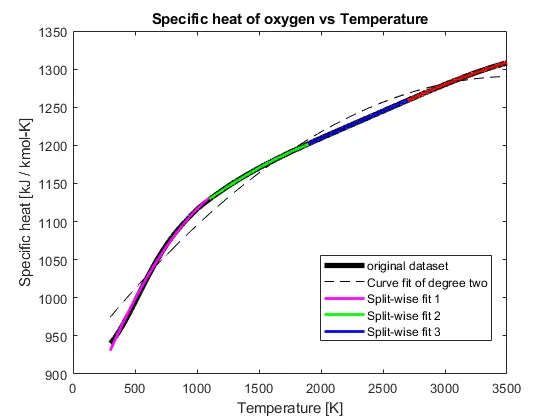
Observation for Split-wise method:

The curve fit for entire graph (dash line) have more deviation than the Split-wise curve fit for the same degree of Polynomial function. This means that by breaking a big data set into small section we can have more accurate curve fit.

Parameter used to measure the Fitness characteristics for both the curves:

Upon finding a curve which satisfies the data points, there are 4 quantities which help us measure the goodness of fit criteria or how well the equation is representing the datapoint. There are.

1. The sum of squares due to errors (SSE)
2. R-Square
3. Adjusted R-Square
4. Root mean squared error (RMSE)

R-Square

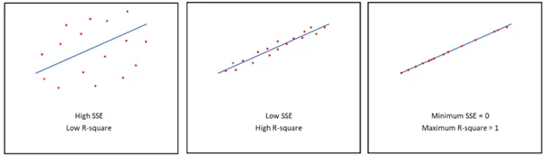
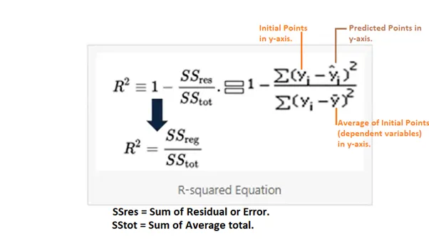
This quantity measures how successful the fit is in explaining the variation of the data. R-Square is the square of the corelation between the response values and the predicted response values.

Higher the R-Square the better the fit, the lower R-Square represents less accurate fit. R-Square ranges from a value 0 to 1.

0 for the worst possible fit for the data set.

1 for the best possible fit for the data set.

Root mean squared error (RMSE)

The root-mean-square deviation (RMSD) or root-mean-square error (RMSE) is a frequently used measure of the differences between values (sample or population values) predicted by a model or an estimator and the values observed.

RMSD is always non-negative, and a value of 0 (almost never achieved in practice) would indicate a perfect fit to the data. In general, a lower RMSD is better than a higher one.

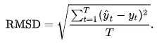
The RMSD of predicted values for times t of a regression's dependent variable with variables observed over T times, is computed for T different predictions as the square root of the mean of the squares of the deviations:

Curve fitting toolbox:

Curve fitting toll box is a great way to get more accurate curve fit. It is simple to use and we can choose from wide range of functions to predict a curve which fits best.

We can also form our own equation to get a desired curve fit for our data.

Furthermore, it also tells us how good our fit is, by providing the values of R-square, adjusted R-square and RMSE.

We can type in the command “cftool” in Command Window to open up Curve fitting toolbox.

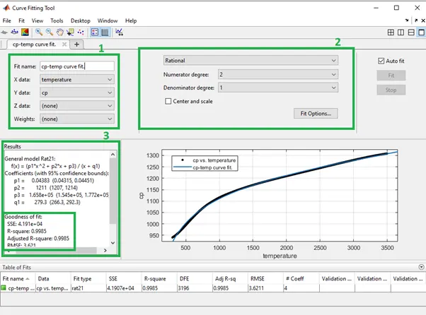
After the Curve fit tool window is open following details are needed to be mentioned in boxes shown above:

1. Mention what X-axis should represent in this case ‘temperature’.

Y-axis represent ‘cp’.

2. Select the type of function.

In this case “Rational” function has been chosen, with numerator degree 2 and denominator degree 1.

3. Box 3, shows the “Rational” function relation and values of four coefficients (p1, p2, p3 & q1).

We can also see the R-Square value is very close to 1, which shows the curve is a good fit.