Challenge

Centrifugal pump design and internal flow analysis using sliding mesh in SolidWorks.

SShubham Dabral13 Aug 2021

Aim

Design and Analysis of a Centrifugal pump.

Objective

To obtain Performance Curve (Relation between net head and volume flow rate) and explain the results obtain.

Introduction

Flow analysis of a rotating region in SolidWorks flow simulation

Take a look at the two examples given below.

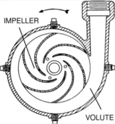
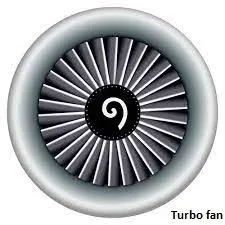
In both the cases, a rotating component rotates around the centre line driving the fluid along with it. The difference between the two cases is that, for the pump impeller, the distance between the impeller and the outer casing varies, this requires us to use a kind of mesh called Sliding mesh. Whereas in turbofan we do not see the variable casing hence we use Local Region Averaging, and this technique is comparatively less time consuming. Therefore, we use Local region averaging for symmetrical casing around the blades and meant for steady state type of analysis.

Centrifugal pump

The word pump is a general term for any fluid machine that adds energy to a fluid. The increase in fluid energy is usually felt as an increase in the pressure of the fluid.

Working:

The shaft driven by a motor drives the impeller. The fluid enters the eye of the impeller and is trapped between the impeller blades. The impeller blades contain the liquid and impart speed to the liquid as it passes from the impeller eye towards the outside diameter of the impeller.

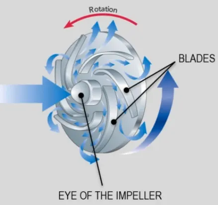
As the fluid acelerate in velocity, a zone of low pressure is generated in the eye of the impeller, confirming the Bernoulli’s principle. The liquid then leves the outer diameter of the impeller and slams the internal casing wall of the volute. At this point the liquid centrifugal velocity comes an abrupt halt and the velocity or kinetic energy is converted into pressure. The pressure further rises when the fluid is conducted from the internal volute housing in an ever increasing escape channel. As the pathway increases the rotory velocity decreases and the pressure increases.

Some fundamental parameters used to analyse the performance of a pump:

Mass flow rate

The mass flow rate, of fluid through the pump is an obvious primary pump performance parameter. For incompressible flow, it is more common to use volume flow rate rather than mass flow rate.

Net head H,

It is the change in Bernoulli head between the inlet and outlet of the pump,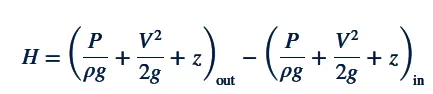

The dimension of net head is length, and it is often listed as an equivalent column height of water, even for a pump that is not pumping water. Net head is proportional to the useful power actually delivered to the fluid.

Pump performance curve

Curves of H, 𝜂pump, and bhp as functions of Volume flow rate are called pump performance curves. The pump performance curves change with rotational speed. An example of a pump performance curves for a centrifugal pump with backward inclined Blades is given below.

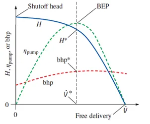
Free delivery is a condition when maximum volume flow rate through a pump occurs. And it occurs when its net head is zero. The free delivery condition is achieved when there is no flow restriction at the pump inlet or outlet—in other words when there is no load on the pump.

Shutoff head is the net head that occurs when the volume flow rate is zero, and is achieved when the outlet port of the pump is blocked off. Under these conditions, net head (H) is large but Volume flow rate is zero.

Note:

For this project, we will trace the performance curve, only, for net Head and Volume flow rate.

Steps Taken

Modelling and Design of a typical Centrifugal pump

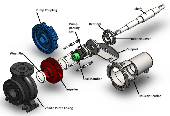
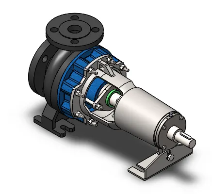
Now creating a solid works flow simulation project

Creating Lids

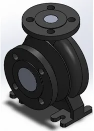
Checking if the geometry is Leak proof by using ‘Leat tracking’.

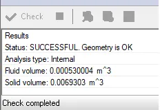
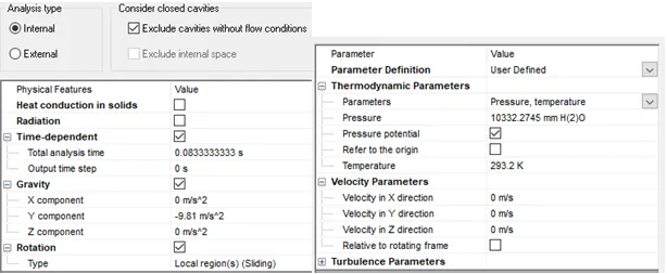
Using flow Wizard to set up internal analysis and input data for our projects.

Creating ‘Rotating Region’ and setting its angular velocity as 1440 RPM (anticlockwise).

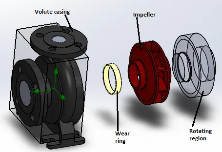
It is important that the ‘Rotating component’ lie compeletly inside the rotating region. Though it may intersect with other components in the assembly.

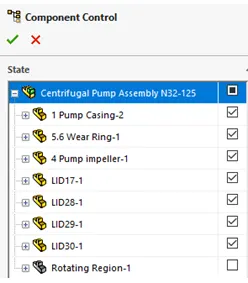
Component Control

Unchecking ‘Rotating region’, so that the software knows that the Rotating Region that we created is not a real wall.

Boundary Condition for case 1

Putting inlet pressure head as environment pressure head and outlet volume flow rate as zero. So that we can obtain the maximum head that the pump can generate at 1440 RPM. By doing this we are trying to simulate ‘Shutoff head’ condition.

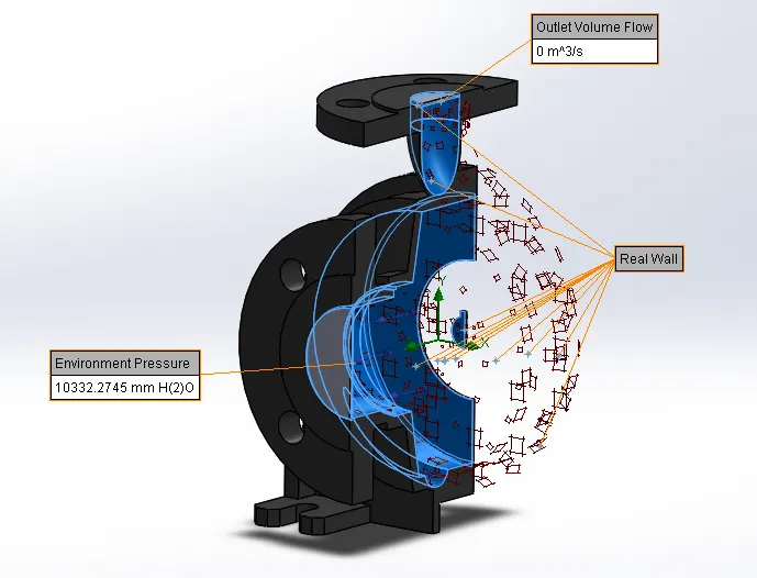
From the data table, we can see that the net head generated by the pump in this case is 18690.04 mm of Water. Also, because of no flow through the outlet the inlet pressure has also increased.

Boundary Condition for case 5

Putting inlet and outlet pressure head equal to environment pressure head to obtain, maximum flow rate. By doing this we are trying to simulate ‘free delivery’ condition.

Even after putting outlet pressure head equal to environment pressure, the outlet pressure has incresed to 16478.23 mm of water. This is because of the work done by the impeller.

Case 5, roughly represents the ‘free delivery’ condition, where outlet pressure is close to inlet pressure. Here, net head (H) is not zero. Hence this condition is close to but not ‘free delivery’ condition. In this case we have obtained a value close to maximum head that is generated by the pump with positive net head. In other words, the pump can provide high flow rate and can push the water to some elevation.

Performing Parametric study

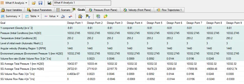
Now to perform parametric study we have two options. First, we can vary the value of head generate by the pump to obtain discharge. Second, we can vary the value of discharge at outlet to obtain the value of pressure head at outlet.

For simplicity, we are going to vary the value of discharge at outlet and record the pressure head generated at the outlet.

For this scernario, we have provided atmosphereic pressure at inlet, Impeller is rotating at 1440 RPM and the suction and discharge diameter remanins constant.

Since, we are varing the discharge volume flow rate, the scenario is analogous to varying the discharge using a valve.

Following data table shows the value of head generated at the outlet when the discharge is increased from 0 to 0.092 m^3/s and then from 0.092 m^3/s to 0.03 m^3/s.

Results and Observations

Data table

Case no.	Suction head [mm H(2)O]	Discharge head [mm H(2)O]	Net Head (H) [mm H(2)O]	Inlet Volume flow rate [m^3/s]	Outlet Volume flow rate [m^3/s]
1	10432.57	29722.61	18690.04	4.4683e-07	0
2	10333.44	27116.61	16783.17	0.0023	0.0023
3	10332.32	22197.70	11865.38	0.0046	0.0046
4	10332.32	21954.90	11622.58	0.0069	0.0069
5	10332.32	16478.23	6145.91	0.0092	0.0092
6	10332.32	3255.69	-7076.63	0.0144	0.0144
7	10332.32	-17859.56	-28191.88	0.0196	0.0196
8	10332.32	-49084.48	-59416.8	0.0248	0.0248
9	10332.32	-93012.74	-103345.06	0.0300	0.0300

Observation

The dischare flow rate and and net head produced by the pump depends on several factors such as Imperller angular speed, impellar diameter, dimension and type of casing,diameter of inlet and outlet etc..
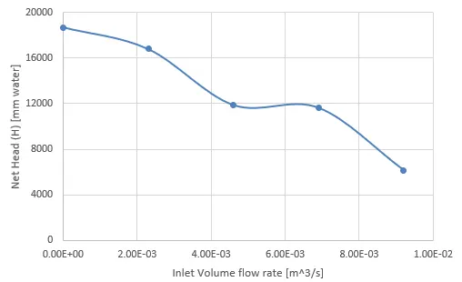
The maximum head generated by the pump is in case 1, when the discharge is zero.
From case 1 to case 5, the net head generated by the pump is positive. And we can observe a general trend that as the Net head (H) decreases the Volume flow rate increases. This means that with increasing flow rate, pump will dischage to lower and lower elevation.
The maximum flow rate is around 0.092 with a net head of 6145.91 mm of water.
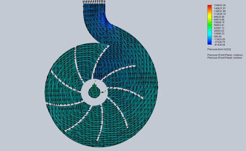
From case 6 to 9 the discharge head value have reduce to a point that it is even lesser than the suction head. This means two things, first, we do not require pump to maintain flow. Second, the software solver is solving for pressure head values with increased discharge rate mathametacially. But it is not able to find any feasible solution. This means that this pump works somewhat in the range from case 1 to case 5 at the provided condition.

Pump performance curve

Cut-plot (for pressure and velocity) & flow trajectory

Case 1

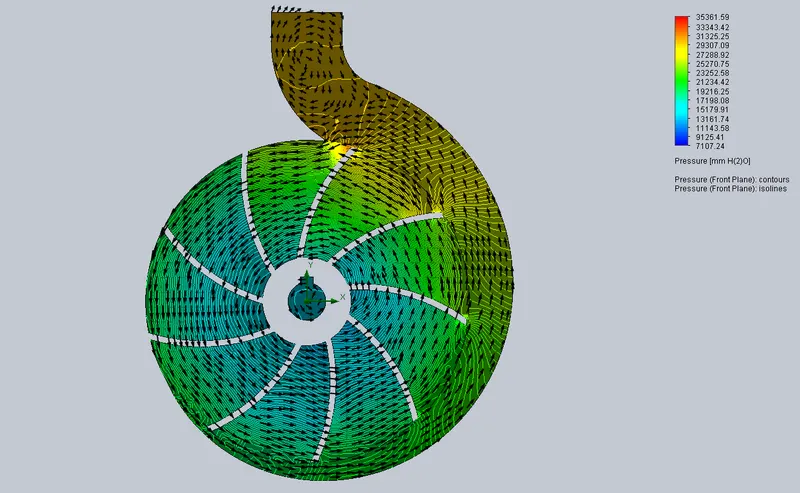
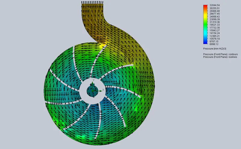
In this case the inlet pressure is atmospheric, impeller rotates at 1440 RPM and the outlet discharge is 0 m^3/s. This case can be visualise as the valve at the outlet being completely shut-off. This case will produce the maximum amount of pressure head at the outlet.

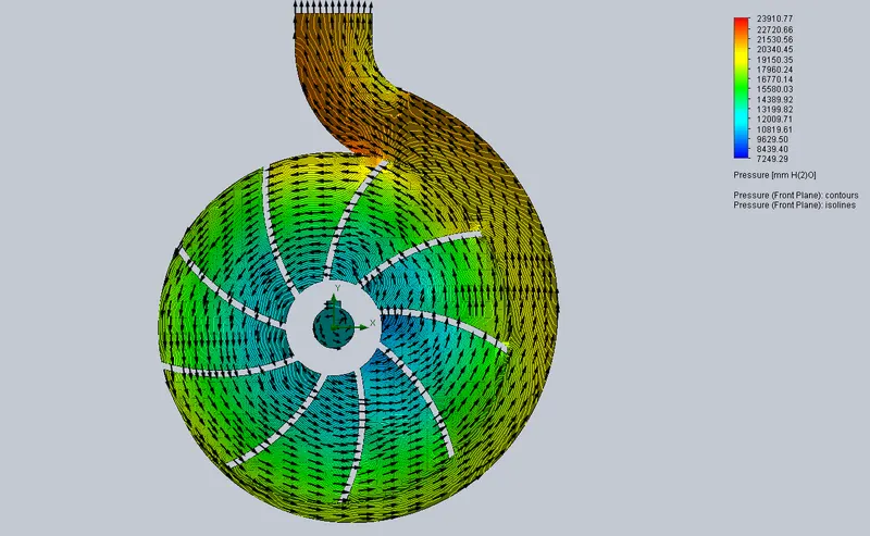
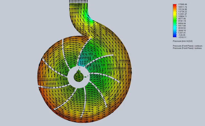
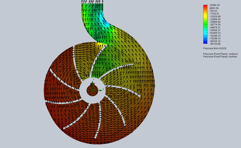
From the pressure plot we can observe the variation of pressure radially using colour code. From the eye of the impeller to the outer diameter of the impeller there is an increase in pressure. The pressure also increases as the fluid moves around the interior of volute casing and reaches its peak at the discharge side of the pump.

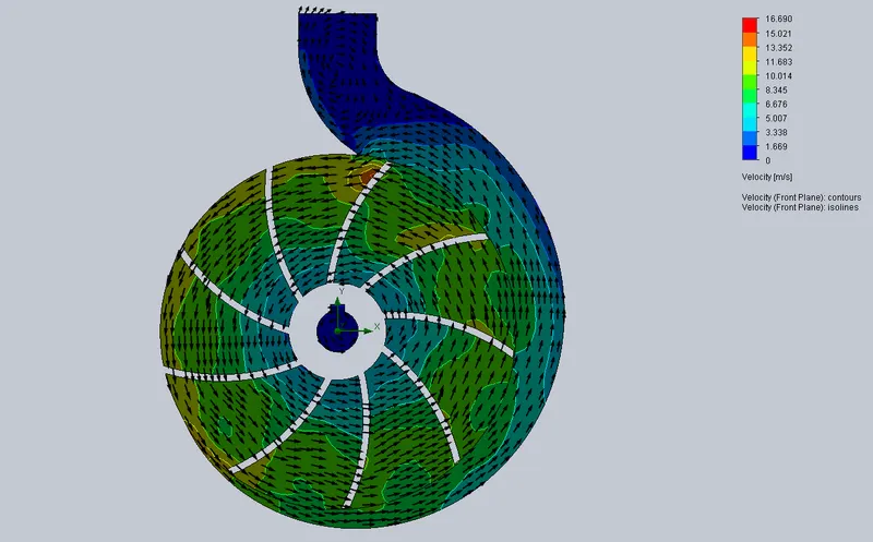
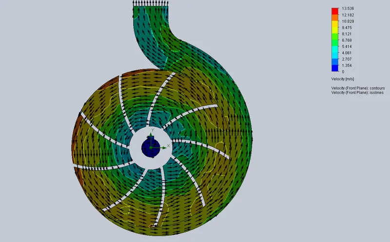
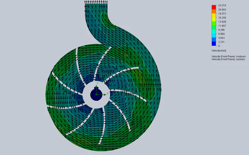
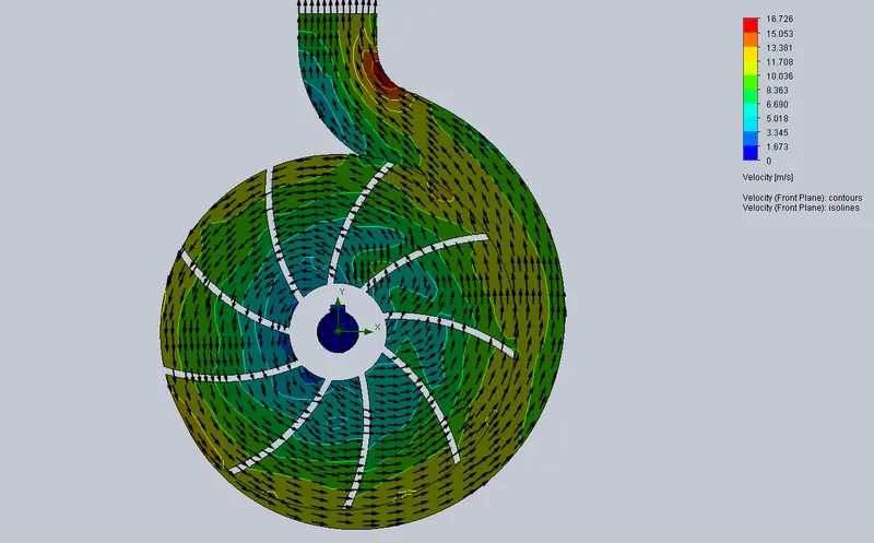
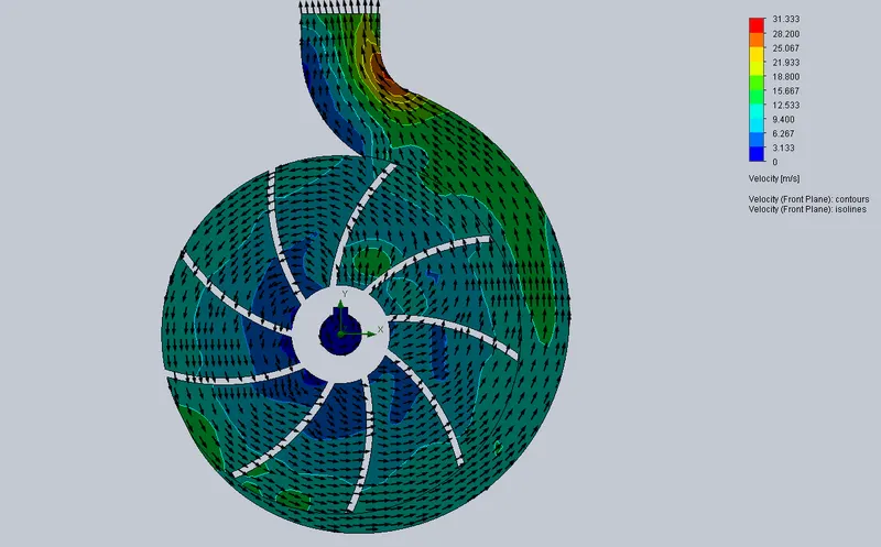
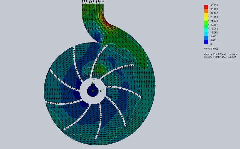
Due to the rotation of the impeller the fluid is also forced to move circular. Hence, the flow velocity of the fluid increases eye of the pump to the outer diameter of the vane. The fluid reaches its peak velocity near the outer diameter of the curved vanes of the impeller where the centrifugal force is maximum. But is starts losing its velocity as it makes contact the inner wall of the casing. The velocity further decreases as it moves along the volute casing of the impeller because of increase in the size of the escape channel. This decrease in velocity is compensated by increase in pressure.

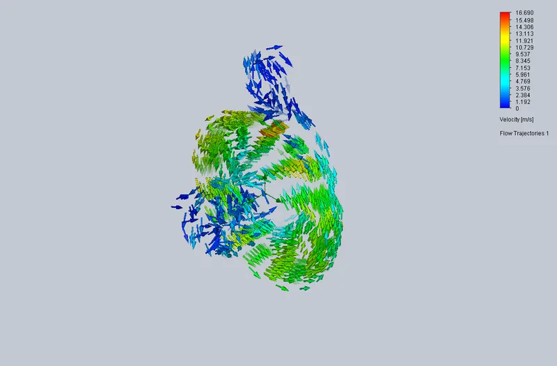
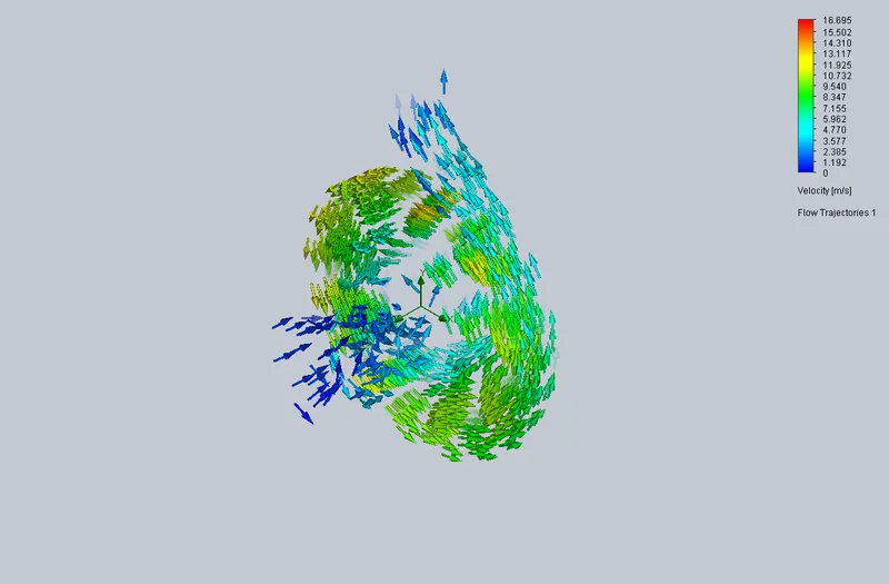
Flow trajectory graph shows how the circular movement of the fluid inside the pump casing takes place. We can also see from colour code how the velocity increases radially. It also shows the reduction in the velocity of fluid as it moves inside the volute and reaches the discharge.

Case 2