Bode plots and Step response
MATLAB commands related to transfer function, pole-zero-gain and step response:
Transfer function:
Transfer function is the ratio of Laplace transformation of output to the Laplace transformation of input.
Transfer function models describe the relationship between the inputs and outputs of a system using a ratio of polynomials. The model order is equal to the order of the denominator polynomial. The roots of the denominator polynomial are referred to as the model poles. The roots of the numerator polynomial are referred to as the model zeros.
The parameters of a transfer function model are its poles, zeros and transport delays.
Commands for Creating Transfer Functions:
Use the commands described in the following table to create transfer functions.
|
Command |
Description |
|---|---|
| tf() |
Create tf objects representing continuous-time or discrete-time transfer functions in polynomial form. |
| zpk() |
Create zpk objects representing continuous-time or discrete-time transfer functions in zero-pole-gain (factorized) form. |
| filt() |
Create tf objects representing discrete-time transfer functions using digital signal processing (DSP) convention. |
| conv() | w = conv(u,v) returns the convolution of vectors u and v. If u and v are vectors of polynomial coefficients, convolving them is equivalent to multiplying the two polynomials. |
Pole-zero-gain:
Use 'zpk' to create zero-pole-gain models, or to convert dynamic system models to zero-pole-gain form.
Zero-pole-gain models are a representation of transfer functions in factorized form. For example, consider the following continuous-time SISO transfer function:
`G(s)`can be factorized into the zero-pole-gain form as:
`G(s)=(s+1)(s−4)(s+2)(s+3).`
A more general representation of the SISO zero-pole-gain model is as follows:
`h(s)=(k(s−z(1))(s−z(2))…(s−z(m)))/((s−p(1))(s−p(2))...(s−p(n))`
Here, z and p are the vectors of real-valued or complex-valued zeros and poles, and K is the real-valued or complex-valued scalar gain
You can create a zero-pole-gain model object either by specifying the poles, zeros and gains directly, or by converting a model of another type (such as a state-space model) to zero-pole-gain form.
You can also use 'zpk' to create generalized state-space models or uncertain state-space (Robust Control Toolbox) models.
Step response:
The step response of a system in a given initial state consists of the time evolution of its outputs when its control inputs areHeaviside step functions. In the control theory, step response is the time behaviour of the outputs of a general system when its inputs change from zero to one in a very short time. The concept can be extended to the abstract mathematical notion of a dynamical system using an evoluation parameter.
Command Description
step, stepplot Plots the step response of all linear and nonlinear models.
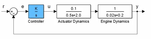
Control system Example for transfer function:
%Transfer function

clear all
close all
clc
%Actuator function
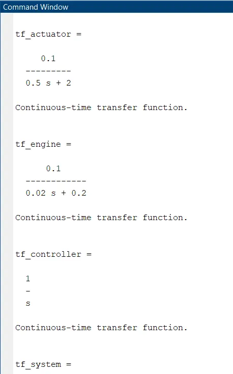
tf_actuator = tf(0.1,[0.5 2])
%Engine function
tf_engine = tf(0.1,[0.02 0.2])
%Controller
tf_controller = tf(1,[1,0])
%System function
tf_system = tf_actuator * tf_engine
%Open loop
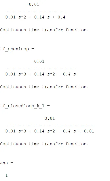
tf_openloop = tf_system * tf_controller
step(tf_openloop)
legend('open loop')
hold on
%Closed loop
tf_closedloop_k_1 = feedback(tf_openloop,1)
%Step response for closed loop
step(tf_closedloop_k_1)
zpk(1)
filt(0.1,[0.5 2])
Procedure:
- Intially defined Actuator function, Engine function, Controller function.
- First calculated system function and open loop.
- Then calculated Transfer function for closed loop.
- Then, plotted the step response for both tthe open loop and closed loop control system.
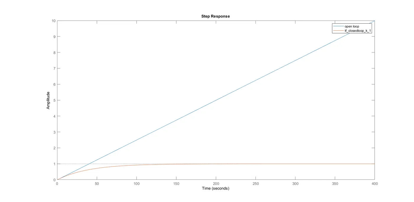
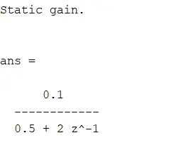
In the closed loop the feedback is taken from the out put and again filter the process. Where as in open loop there is no feedback is taken hence the amplitude is increased linearly.
2.For the unity feedback system shown in figure below. Determine closed loop step response using MATLAB commands. Comment on the result.
`G(s)=(30(s2-5s+3))/((s+1)(s+2)(s+4)(s+5))`
By solving the above equation we get
`G(s)=(30s2-150s+90)/(s4+12s3+49s2+78s+40)`
Calculated step response by using MATLAB code:
%Transfer function_2
clear all
close all
clc
%Inputs
num=[30 -150 90]
dem=[1 12 49 78 40]
%Transfer function
G=tf(num,dem)
%Step response
step(G)
grid on
Procedure:
- Initially defined the inputs of numerator and denominator variables.
- Next, by using the 'tf()' command created a transfer function for the given variables.
- Then, plotted the bode plot of defined Transfer function.
Results:
Step response of a given Transfer function is
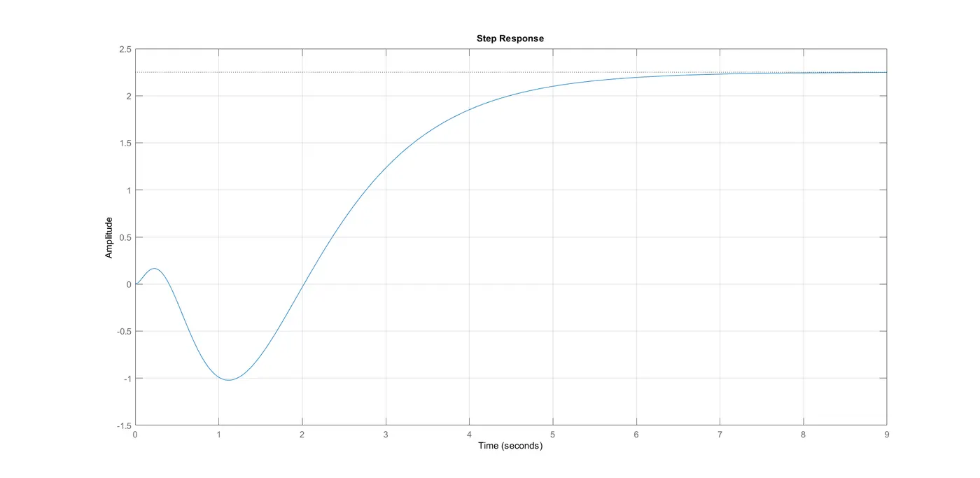
- Starting the Amplitude is damped and decreased to -1 during the 0 to 1.2 sec and then gradually increased and after 8 seconds the amplitude attended to 2.25
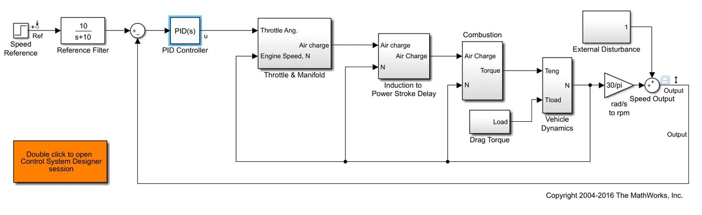
3. Explain the MATLAB model scdspeedctrl . Comment on results for non-tuned PID gain values.
Design Overview:
This example introduces the process of designing a single-loop control system with both feedback and prefilter compensators. The goal of the design is to:
Track the reference signal from a Simulink step block scdspeedctrl/Speed Reference. The design requirement is to have a settling time of under 5 seconds and zero steady-state error to the step reference input.
Reject an unmeasured output disturbance specified in the subsystem scdspeedctrl/External Disturbance. The design requirement is to reduce the peak deviation to 190 RPM and to have zero steady-state error for a step disturbance input.
In this example, the stabilization of the feedback loop and the rejection of the output disturbance are achieved by designing the PID compensator scdspeedctrl/PID Controller. The prefilter scdspeedctrl/Reference Filter is used to tune the response of the feedback system to changes in the reference tracking.
Open Control System Designer
This example uses Control System Designer to tune the compensators in the feedback system. To open the Control System Designer
Launch a pre-configured Control System Designer session by double-clicking the subsystem in the lower left corner of the model.
Configure Control System Designer using the following procedure.
Open Control System Designer:
This example uses Control System Designer to tune the compensators in the feedback system. To open the Control System Designer
Launch a pre-configured Control System Designer session by double-clicking the subsystem in the lower left corner of the model.
Configure Control System Designer using the following procedure.
Tune Compensators:
Control System Designer contains several methods tuning a control system:
Manually tune the parameters of each compensator using the compensator editor. For more information, see Tune Simulink Blocks Using Compensator Editor.
Graphically tune the compensator poles, zeros, and gains using open/closed-loop Bode, root locus, or Nichols editor plots. Click Tuning Methods, and select an editor under Graphical Tuning.
Optimize compensator parameters using both time-domain and frequency-domain design requirements (requires Simulink Design Optimization™ software). Click Tuning Methods, and select Optimization based tuning. For more information, see Enforcing Time and Frequency Requirements on a Single-Loop Controller Design (Simulink Design Optimization).
Compute initial compensator parameters using automated tuning based on parameters such as closed-loop time constants. Click Tuning Methods, and select either PID Tuning, Internal Model Control (IMC) Tuning, Loop Shaping (requires Robust Control Toolbox™ software), or LQG Synthesis.
Design:
The following compensator parameters satisfy the design requirements:
scdspeedctrl/PID Controller has parameters:
P = 0.0012191
I = 0.0030038
scdspeedctrl/Reference Filter:
Numerator = 10
Denominator = [1 10]
The responses of the closed-loop system are shown below
Non-tuned PID gain:
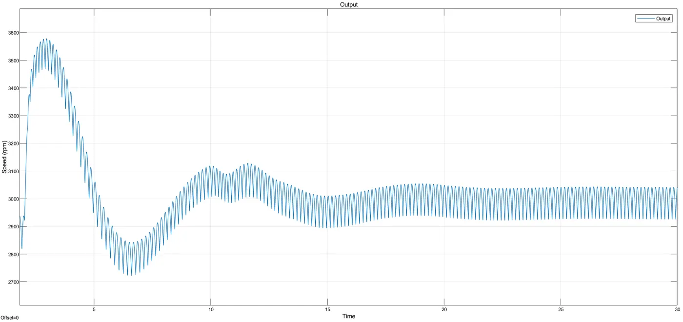
Before tuning there is a fluctuation of speed (rpm).
Tuned and updated:
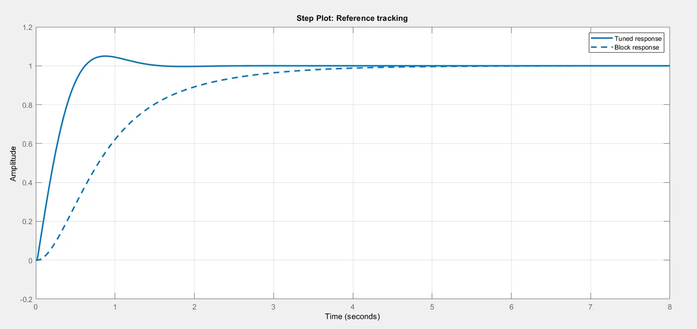
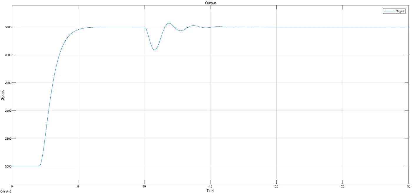
After tuning the fluctuation of output rpm is reducded and curve is smooth. only from time 10 secto 17 sec the speed is fluctuated between 2700 to 3100 rpm.
4.What is the importance of bode plot for control system design? Using MATLAB make a bode plot of transfer function
Importance of bode plot for control system design:
- In electrical engineering and control theory, a Bode plot is a graph of the frequency response of a system. It is used to determine the stability of a control system. It is usually a combination of a Bode magnitude plot (expressing the magnitude in decibels) of the frequency response, and a Bode phase plot (expressing the phase shift in degrees).
- Frequency response of an electric or electronics circuit allows us to see exactly how the output gain (magnitude response) and the phase (phase response) changes at a particular single frequency, or over a whole range of different frequencies from 0Hz, (d.c) to many thousands of mega-hertz, (MHz).
- Generally, the frequency response analysis of a circuit or system is shown by plotting its gain, that is the size of its output signal to its input signal (Output/Input), against a frequency scale over which the circuit or system is expected to operate. Graphical representations of frequency response curves are called Bode plots and as such Bode plots are generally said to be semi-logarithmic graphs because one scale (X-axis) is logarithmic and the other (Y-axis) is linear.
MATLAB code for plotting bode plot of Transfer function:
%Bode plot
clear all
close all
clc
num=[2 5]
dem=[1 12 20 0]
h=tf(num,dem)
bode(h)
grid on
Procedure:
- Initially defined the inputs of numerator and denominator variables.
- Next, by using the 'tf()' command created a transfer function for the given variables.
- Then, plotted the bode plot of defined Transfer function.
Results:
Bode plot for `h=(2s+5)/(s3+12s2+20s)` is
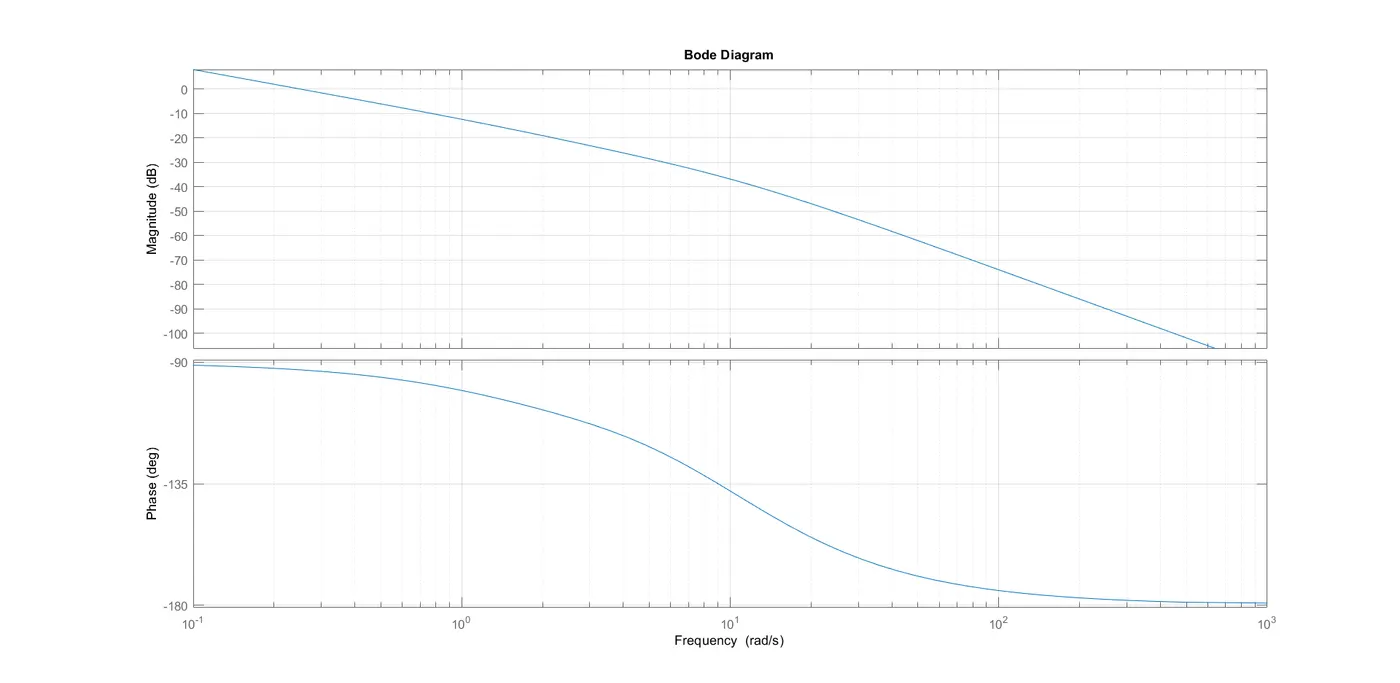
In the bode plot the magnitude (dB) reduced to -ve values and the phase (deg) reduced from -90 to 180 deg
Concusion:
Hence, the Bode plot of Transfer function is plotted.