Basics of ML & AL Week 2 Challenge
1. Calculate all 4 business moments using pen and paper for the below data set?
First Business Moment - Mean:
`mu = sum(X_i*P(X))`
`mu = (0 times0.35)+(1 times0.25)+(2 times0.15)+(3 times0.15)+(4 times0.10)`
`mu = 0+0.25+0.30+0.45+0.4`
`mu=1.4`
Second Business Moment - Variance:
`sigma^2 = sum(X_i-mu)^2*P(X)`
`sigma^2 = (0-1.4)^2 * 0.35+(1-1.4)^2 * 0.25+(2-1.4)^2 * 0.15+(3-1.4)^2 * 0.15+(4-1.4)^2 * 0.10`
`sigma^2 = 0.686+0.04+0.054+0.384+0.676`
`sigma^2 = 1.84`
`sigma = 1.36`
Third Business Moment - Skewness:
`S_k = sum((X_i-mu_x)/sigma)^3*P(X)`
`S_k = ((0-1.4)/1.36)^3*0.35+((1-1.4)/1.36)^3*0.25+((2-1.4)/1.36)^3*0.15+((3-1.4)/1.36)^3*0.15+((4-1.4)/1.36)^3*0.10`
`S_k = (-0.38)+(-0.006)+0.0129+0.2442+0.6987`
`S_k = 0.57`
Fourth Business Moment - Kurtosis:
`K_t = sum((X_i-mu_x)/sigma)^4*P(X) - 3`
`S_k = ((0-1.4)/1.36)^4*0.35+((1-1.4)/1.36)^4*0.25+((2-1.4)/1.36)^4*0.15+((3-1.4)/1.36)^4*0.15+((4-1.4)/1.36)^4*0.10-3`
`K_t = 0.393+0.00187+0.00568+0.287+1.3358-3`
`K_t = -0.98`
2)What is the significance of expected value when simple mean (Sum of all observations/number of observations) is already in place
An expected value gives a quick insight into the behavior of a random variable without knowing if it is discrete or continuous.
Therefore, two random variables with the same expected value can have different probability distributions. Other descriptive measures like standard deviation also affect the shape of the distribution. The expected value of a random variable X is denoted as E(X).
Let’s say that X is a discrete random variable with possible values x1, x2, x3, … , xn. Also, p(xi) denotes P(X = xi). Therefore, the expected value of X is:
μ = E(X) = Σp(xi) – xi … where the elements are summed over all the values of the random variable X.
If X is a continuous random variable with a probability density function f(x), the the expected value of X is:
μ = E(X) = ∫x.f(x)dx
3)Having skewness in the curve considered to be bad in the analysis?
Skewness refers to distortion or lack of symmetry in a symmetrical bell curve, or normal distribution in a set of data. If the curve is shifted to left or right, it is said to be skewed. Skewness can be qualified as a representation of the extent to which a given distribution varies from a normal distributution. A normal distribution has a skew of zero.
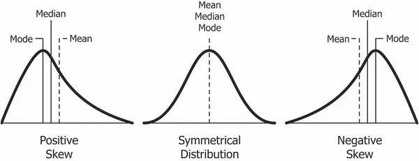
Skewed data can often lead to skewed residuals because "outliers" are strongly associated with skewness, and outliers tend to remain outliers in the residuals, making residuals skewed. But technically there is nothing wrong with skewed data. It can often lead to non-skewed residuals if the model is specified correctly.
Mean : Average of the data sets
Median : Central value in the data sets
Mode : Repeating number in the data set
4)Evaluate the probabilities for continuous normal distribution with given mean = 680 and standard deviation = 31
a)P(X<711)
b)P(X>740)
c)P(600<x<720)
d)P(X=720)
To evaluate the probalities for continuous and normal distribution will use "Z- formula" and "Z-Table".
`Z = (X-mu)/sigma`
Where `X=`Random variable
`Mean (mu) = 680`
`S.D(sigma) = 31`
a)P(X<711):
`Z = (711-680)/31`
`Z=1`
`P(Z<1) = 0.8413` from the Z-Table.
This is the area to the left of the Z score, since X is less than 711.
b)P(X>740):
`Z=(740-680)/31`
`Z=1.94`
`P(Z>1.94) = 0.9738`
This is the area to the left of the Z score, but we need to calculate the area to the right of the Z score,
`P(Z>1.94) = 1- P(Z<1.94)`
`P(Z>1.94) = 0.0287`
c)P(600<x<720):
`Z=(600-711)/31 & Z=(720-711)/31`
`Z=-2.58 & Z =1.29`
We need to find the area for the Z score -2.58 and 1.29 subtract the values to get the probability.
P(-2.58<Z1.29) = P(Z<1.29)-P(Z<-2.58)
P(-2.58<Z1.29) = 0.9032-0.0047
P(-2.58<Z1.29) = 0.89854
d)P(X=720):
`Z =1.29`
`P(Z=1.29) =0.9015`
`P(Z=1.29) = 0.9015-0.9015`
`P(Z=1.29) = 0`
5)Explain the curve on the right side.
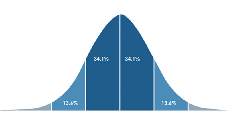
- `1 sigma`(S.D) from the mean is around 34.1 either side of the mean and hence the values lies b/w -34.1% and 34.1% = 68.2% of values falles in the 1 S.D
- `2 sigma`(S.D) from the mean is taken as 34.1+34.1+13.6+13.6= 95.4% approximately the values fales in the 2S.D from the mean.
- `3 sigma` from the mean is taken as 34.1+34.1+13.6+13.6+2.1+2.1 = 99.7% approximately the values falls in the 3S.D from the mean.