Comparison of simulation using different contact types and notches in RADIOSS

OBJECTIVE: To perform analysis of crush tube crashing on rigid wall using different parameters. To compare and contrast the variation in results occurring due to change in parameters. To perform mesh on given bumper model.

PROCEDURE:

To complete the meshing of the bumper model, the following steps have to be followed:

1. Perform geometrical cleanup.

2. Perform 2D meshing

3. Create 1D connectors to join the various parts

To complete the analysis of the simulation, the following steps have to be followed:

1. Import the .rad file into Hypermesh.

2. Do the necessary variations as required in the assignment

3. Export the changed simulation to a separate .rad file.

4. Run the simulation and plot the necessary graphs

5. Make a comparison for the variation in values between the different simulation cases and make conclusions

1. Meshing of bumper model:

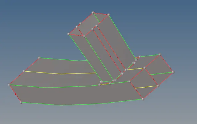
The bumper model is first imported into Hypermesh and geometric cleanup was done. The final geometry before meshing is given below:

To mesh the geometry with 2D shell elements, go to 2D => automesh.

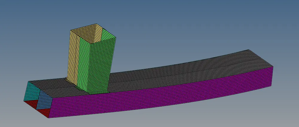
The following image shows the bumper model after 2D meshing was completed:

To add 1D elements, go to 1D => connectors => spot and add spot welds to unconnected parts.

Thus, the bumper model was successfully meshed.

The crash simulation is split into 6 cases and the results are given below.

CASE 1: NO CHANGE:

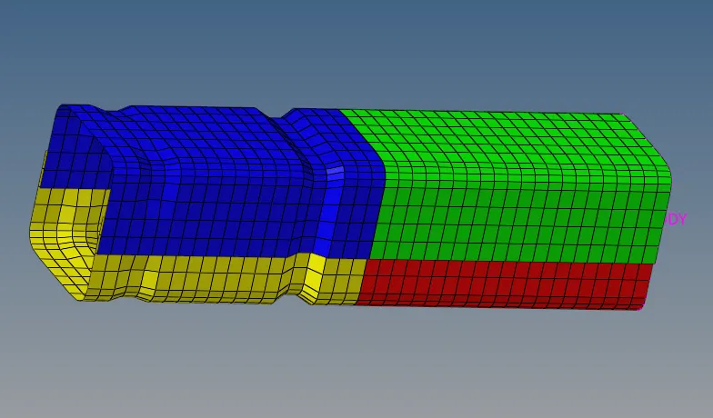
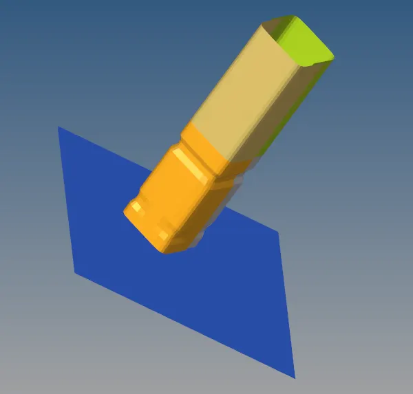
In the first case, the given model is simulated using RADIOSS without making any changes. To begin the simulation, go to Analysis => RADIOSS. The simulation file with the crush tube FE elements are rigid wall are shown below:

The simulation results of the first case are given below:

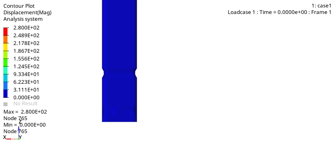
DISPLACEMENT VARIATION

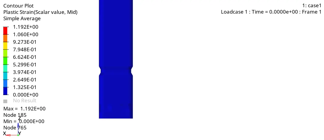
STRAIN VARIATION

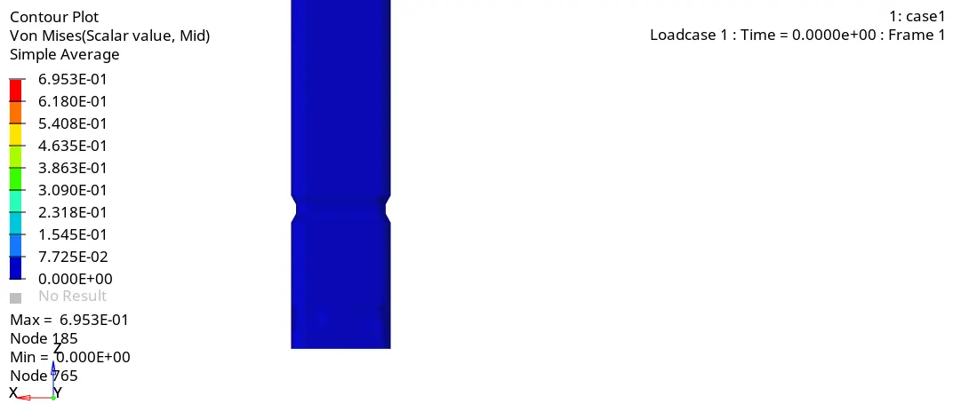
STRESS VARIATION

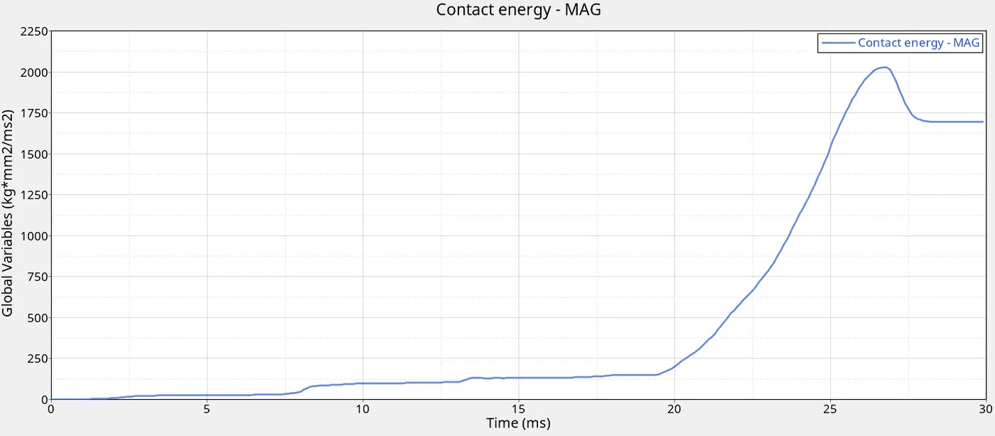
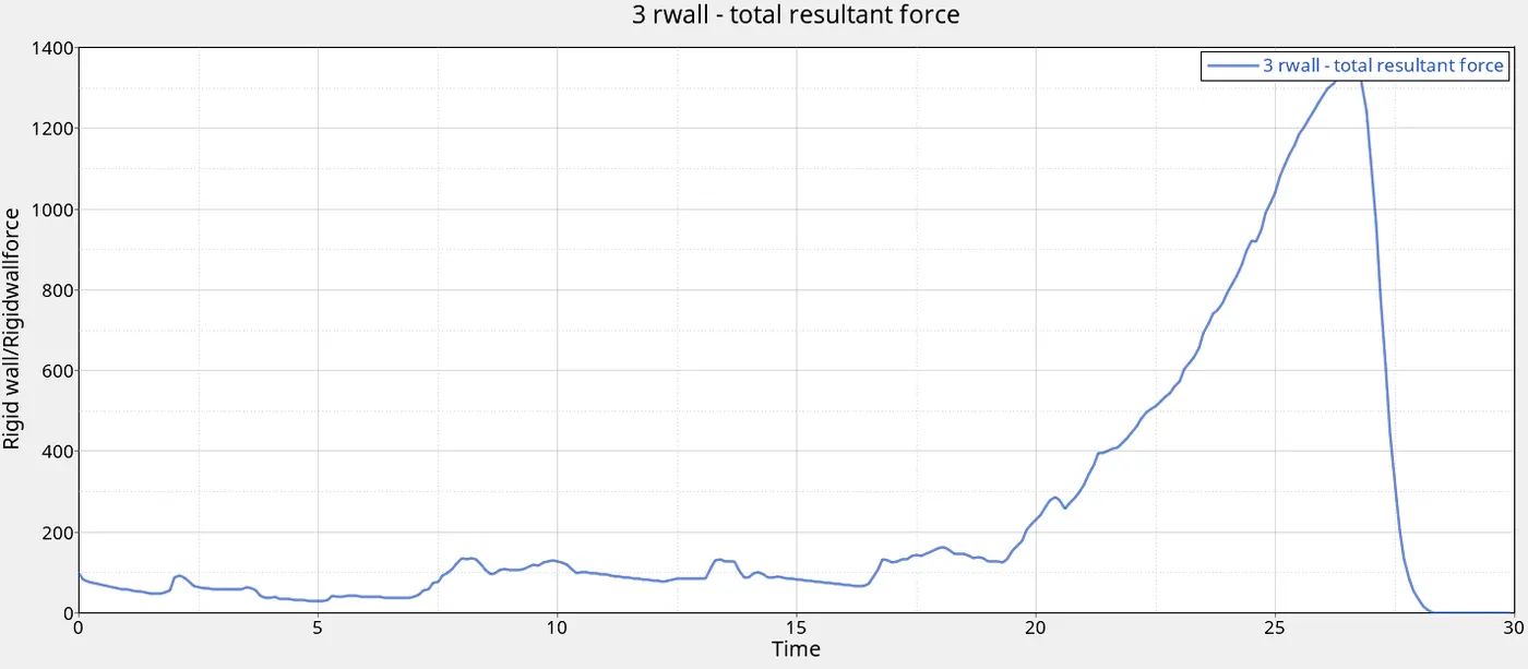
CASE 2: Change Inacti to 6:

The value for Inacti is changed from 0 to 6. This removes initial penetrations if possible and adjusts gap. To accomplish this, edit the self contact card and change the Inacti value. The following results were obtained:

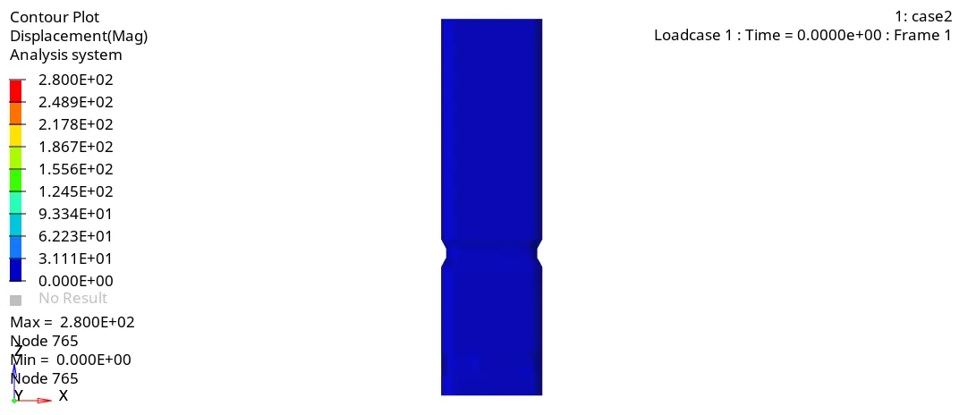
DISPLACEMENT VARIATION

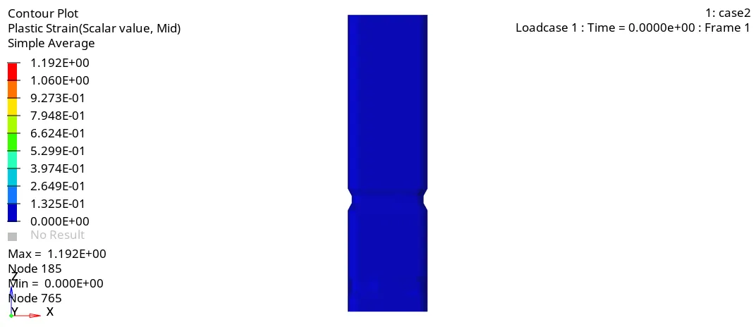
STRAIN VARIATION

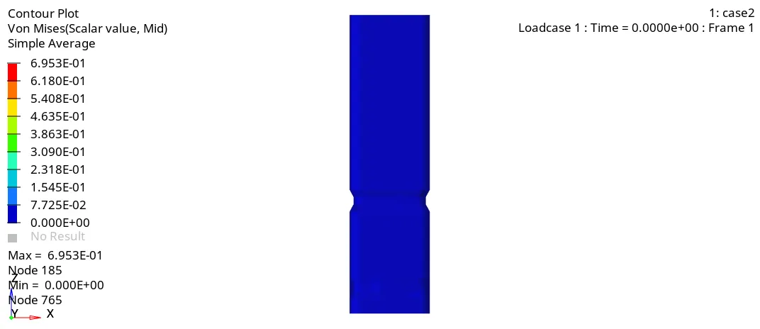
STRESS VARIATION

CASE 3: Change contact type to Type 11:

Type 11 contact enables solution to edge-to-edge contact which when working in tandem with type 7 contact which is node-to-surface contact, gets the more accurate result. To accomplish this, create a new contact card and change it to Type 11 and select the appropriate parts to establish the contact. The following results were obtained:

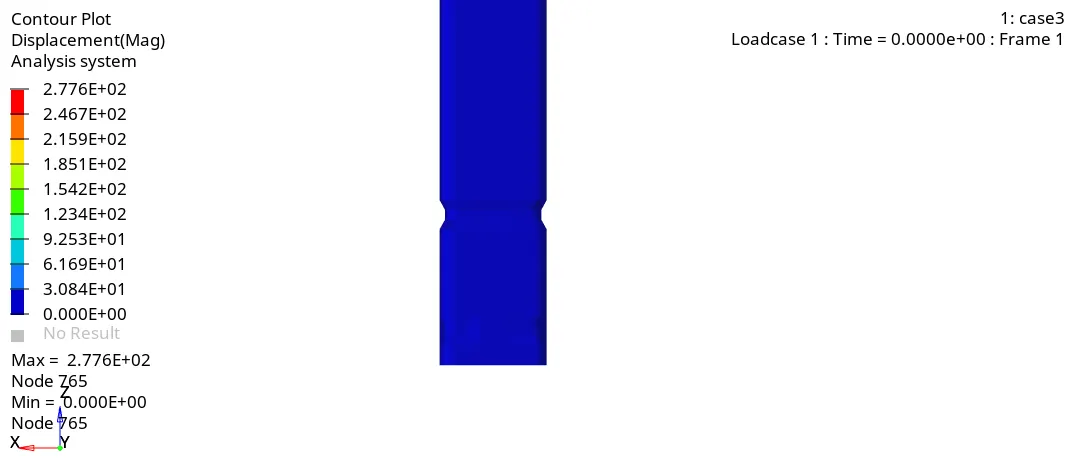
DISPLACEMENT VARIATION

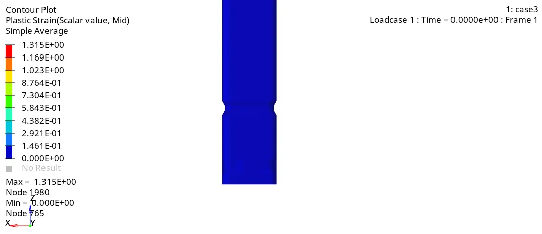
STRAIN VARIATION

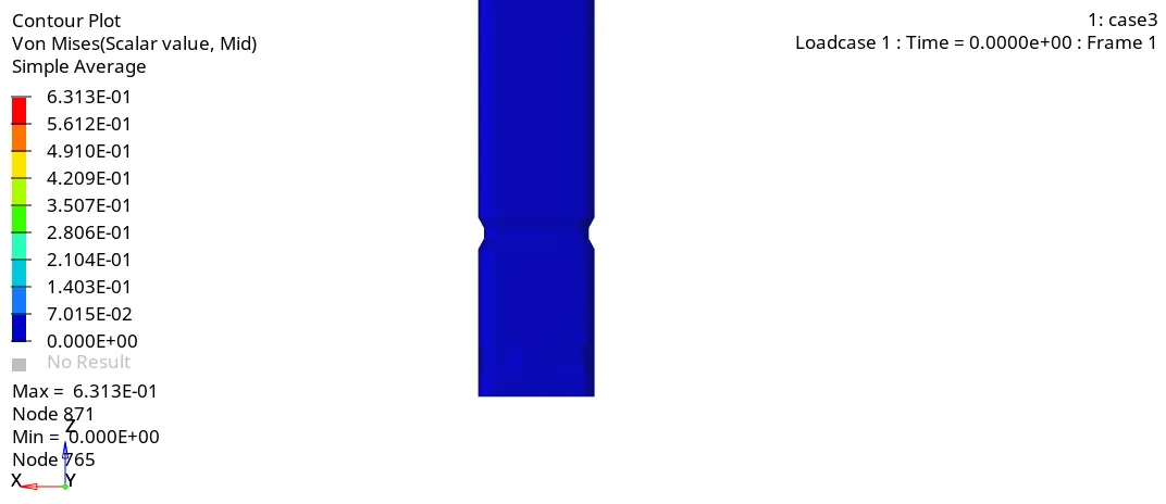
STRESS VARIATION

CASE 4: Remove the two notches and remove the boundary condition on rigid body:

To remove the two notches, nodes of the notches were made to align with the nodes of the flat regions. This was done by going to GEOM => node edit => align node.

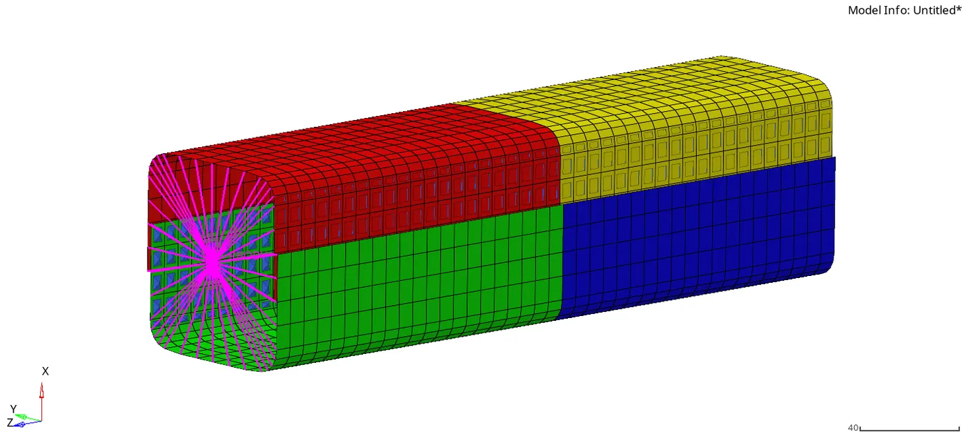
The first and second end are selected from the flat surface and then the nodes of the notches are selected and aligned. This flattens the notch region. The boundary conditions were removed by going to Solver and the boundary condition card was changed and all the dofs were unticked which means that they are free to move in all 6 motions. The tube after the alignment procedure is shown below:

The results of the simulation are given below:

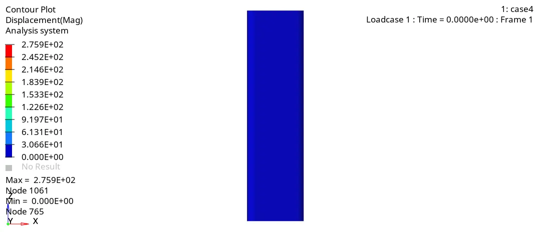
DISPLACEMENT VARIATION

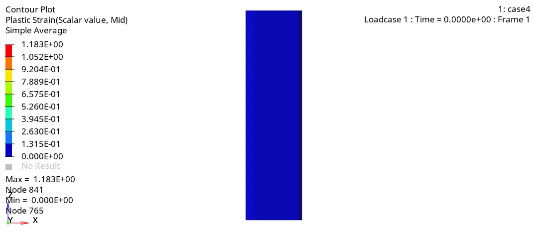
STRAIN VARIATION

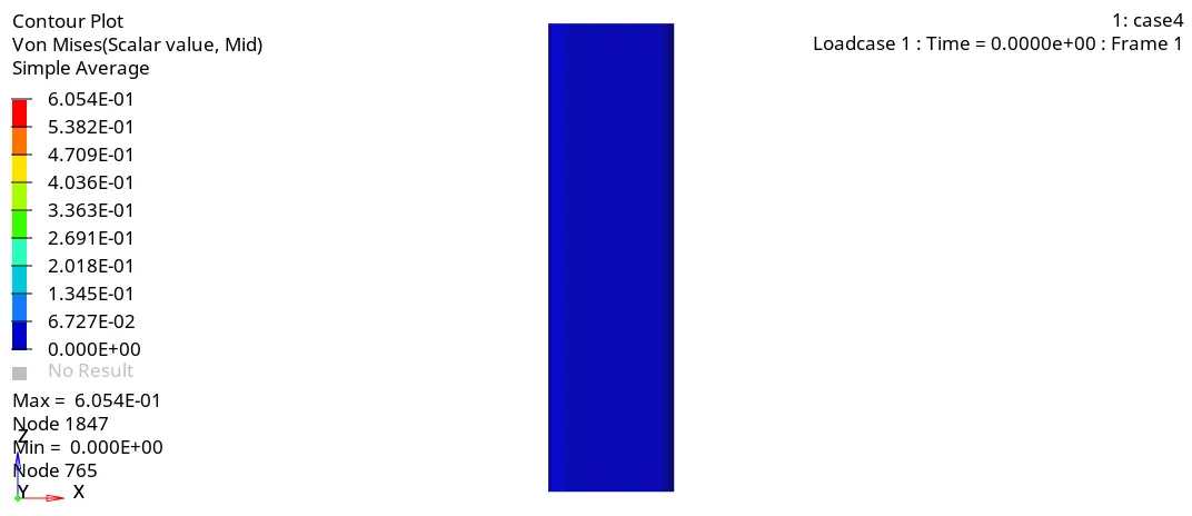
STRESS VARIATION

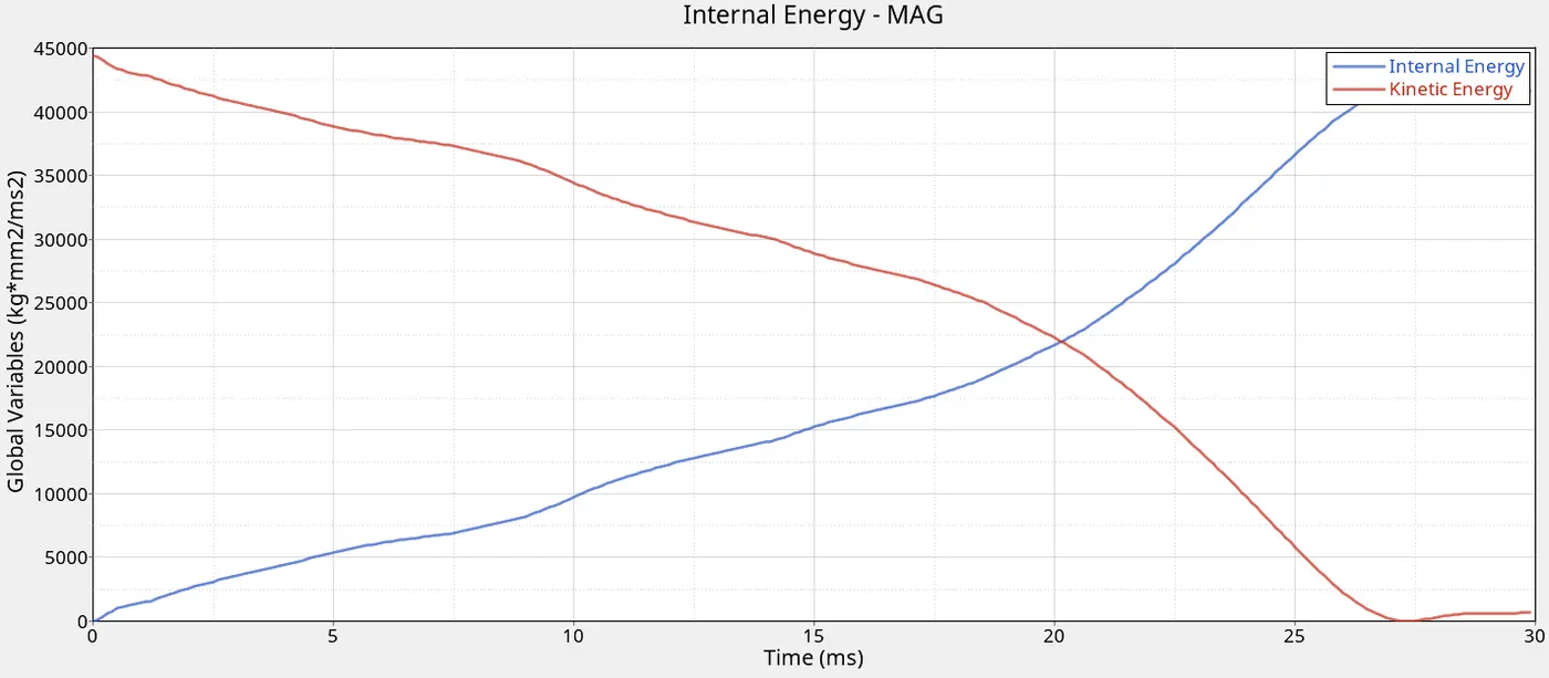
CASE 5: Create a notch in the middle:

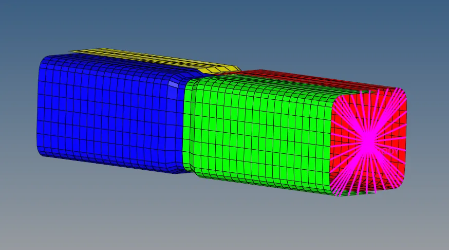
To create a notch in the middle, the element are offset by using 2D => elem offset.

The model was changed and is given below:

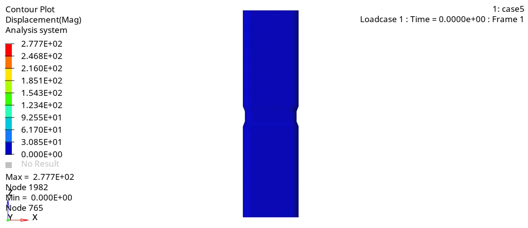
The results obtained are given below:

DISPLACEMENT VARIATION

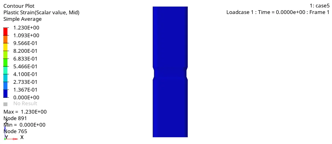
STRAIN VARIATION

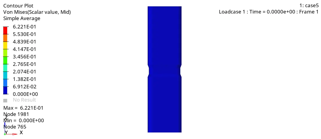
STRESS VARIATION

CASE 6: Create a new notch only on opposing two faces:

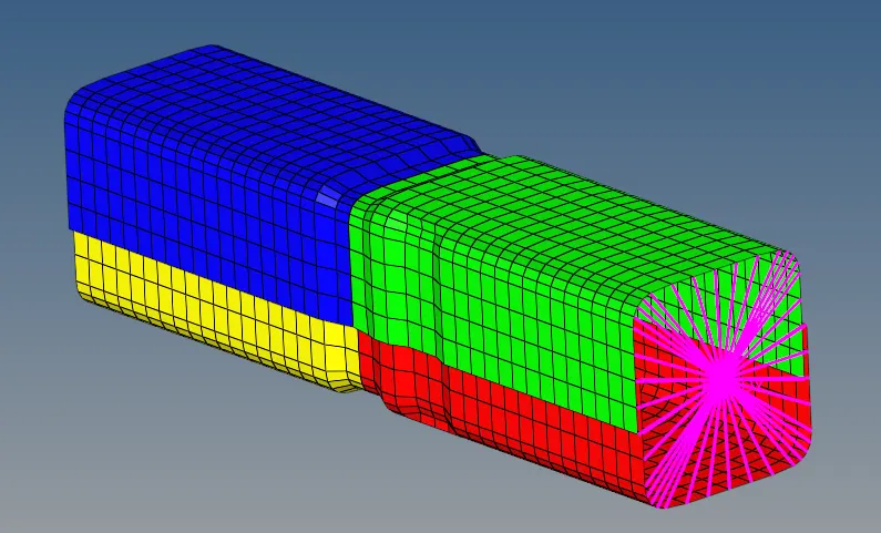
Similar to case 5, the notch was created using element offset but only on two opposing faces. The model is given below:

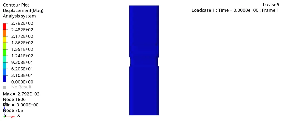
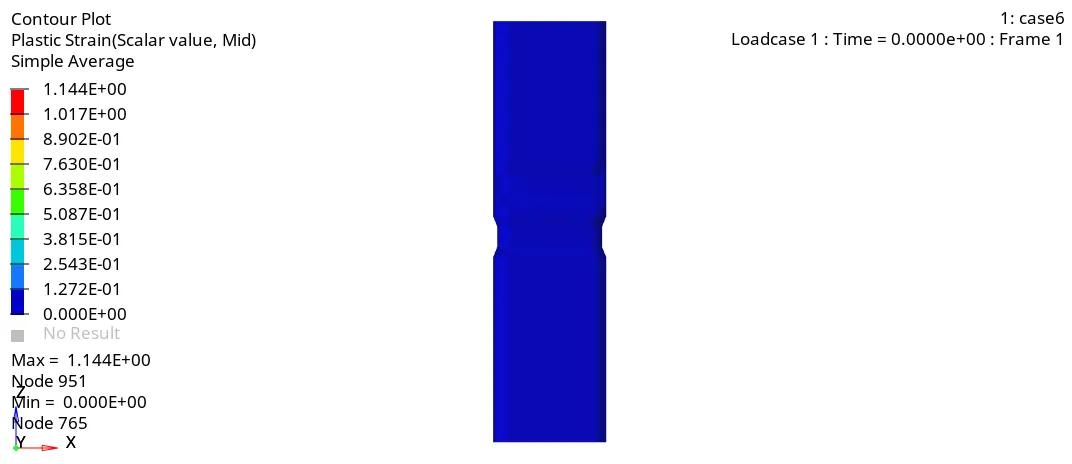
The results of the simulation are given below:

DISPLACEMENT VARIATION

STRAIN VARIATION

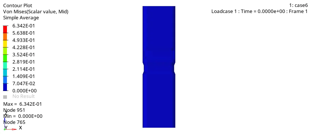
STRESS VARIATION

COMPARISON OF RESULTS:

Apart from the graphs and .gif files given above, some important parameters extracted from the simulation of the six cases are tabulated below:

Parameters	Case 1	Case 2	Case 3	Case 4	Case 5	Case 6
Elapsed Time (s)	124.48	161.05	250.06	220.7	250.69	268.36
Energy error	-4.6%	-4.6%	-6.2%	-5.5%	-4.8%	-6.2%
Maximum Internal Energy (J)	42020	42020	41350	41690	41810	41260
Maximum Displacement (mm)	280	280	277.6	275.9	277.7	279.2
Maximum Strain	1.192	1.192	1.315	1.183	1.23	1.144
Maximum Stress (MPa)	0.6953	0.6953	0.6313	0.6054	0.6221	0.6342
Maximum Contact forces (KN)	93.82	93.82	360.3	522.4	361.2	559.6
Maximum rigid wall force (KN)	1300	1390	1480	1180	1310	1320

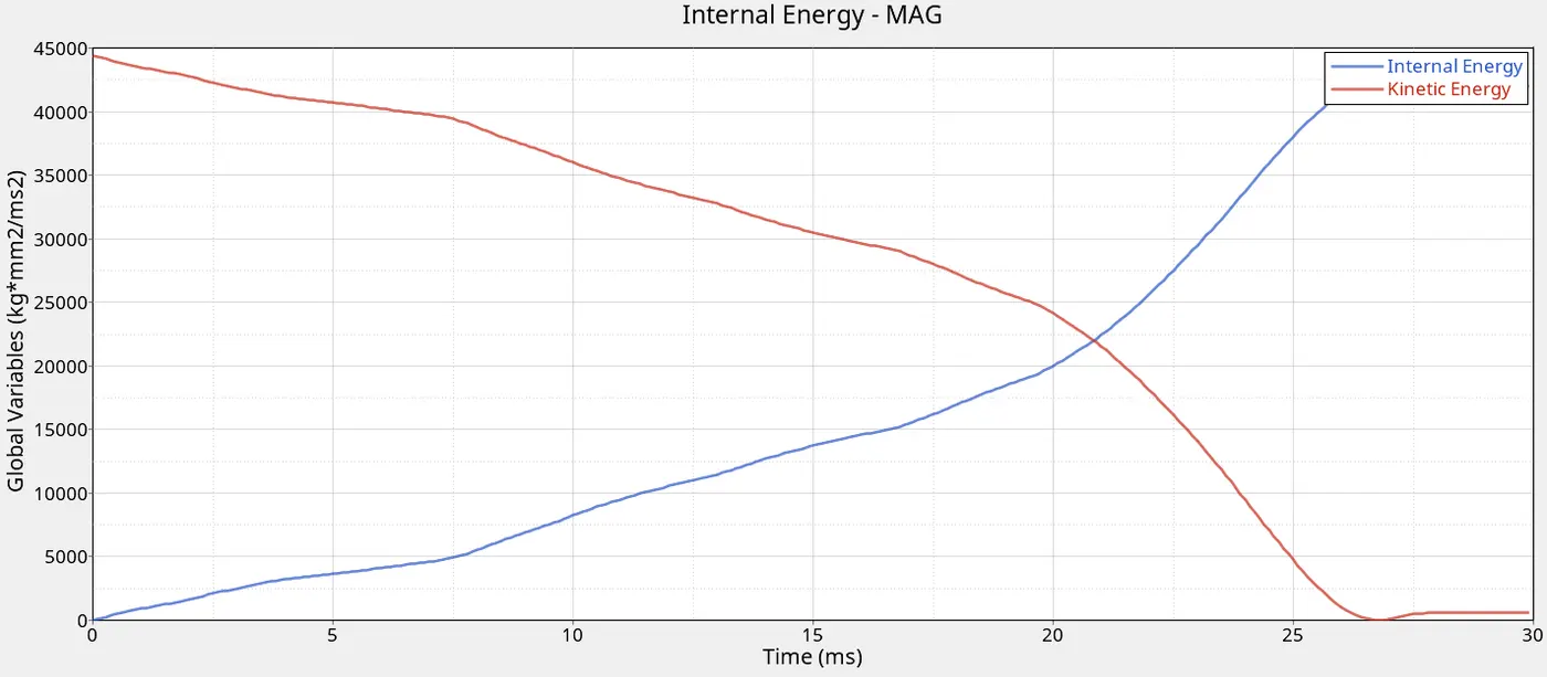
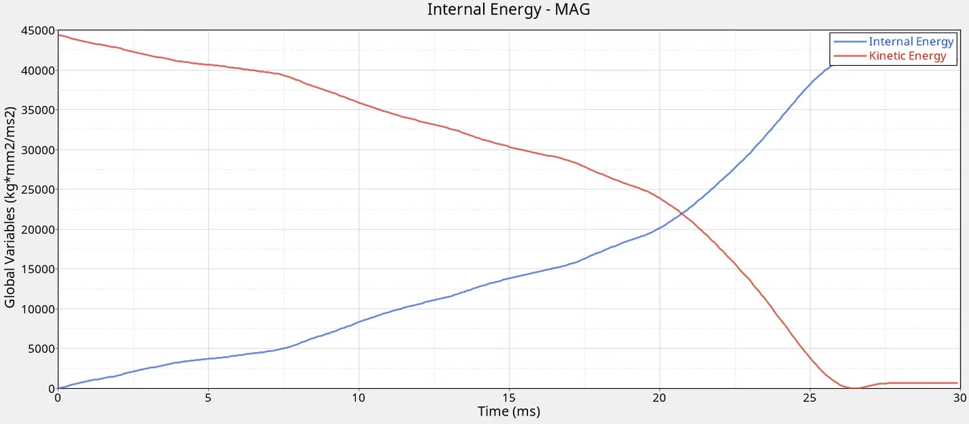
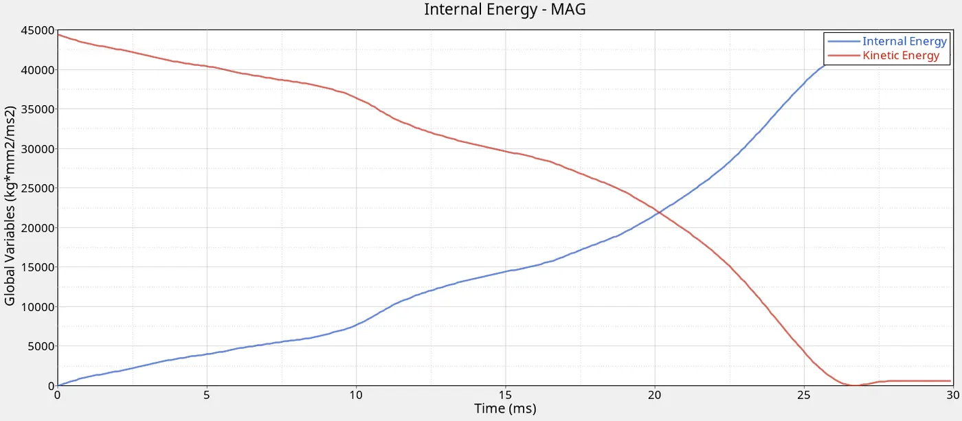
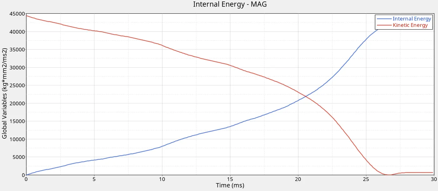
The graphs which were given for each case are more or less similar to each other with minor variations in peak values. In each case the internal energy increases from zero at beginning to peak at the end, whereas the kinetic energy is at peak at the beginning and as time moves forward, the kinetic energy keeps reducing. This is because the kinetic energy of the tube when it crashes on to the rigid wall causes the velocity to reduce to zero eventually. This energy is dissipated partially into the material in the form of internal energy.

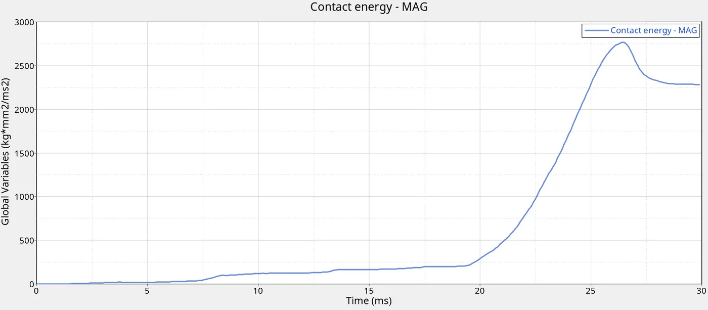
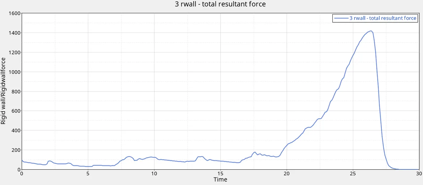
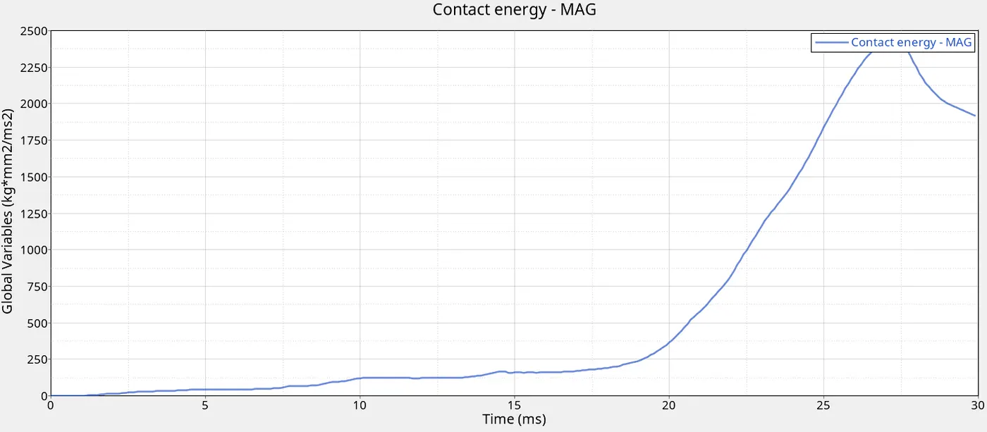
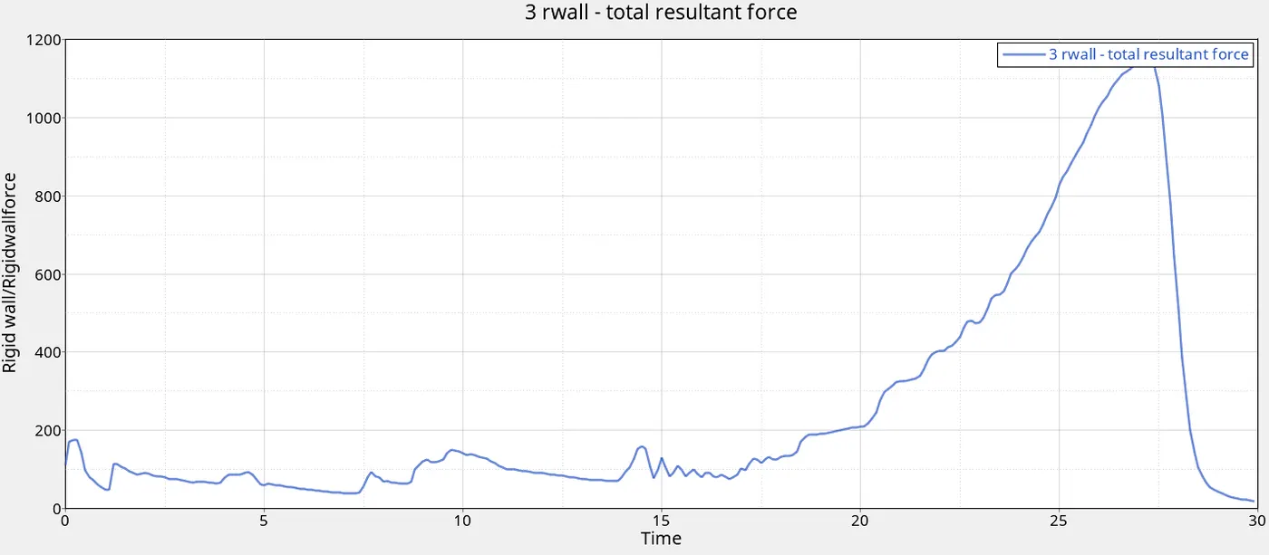
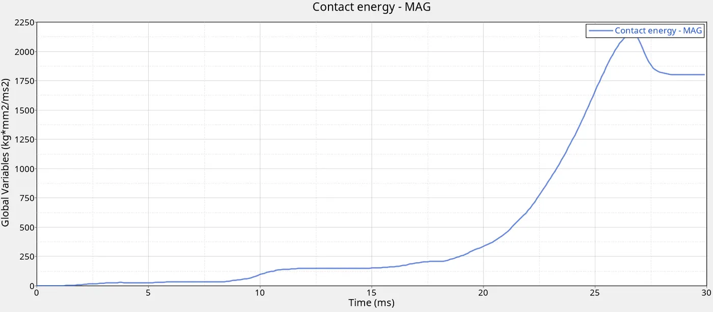
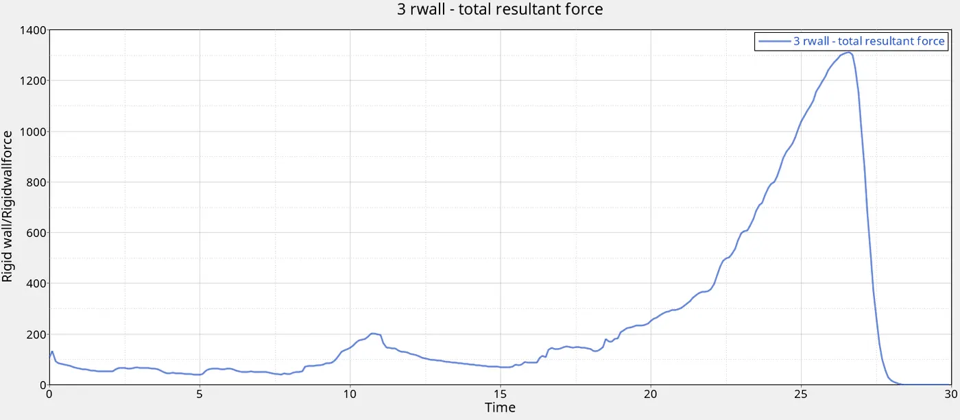
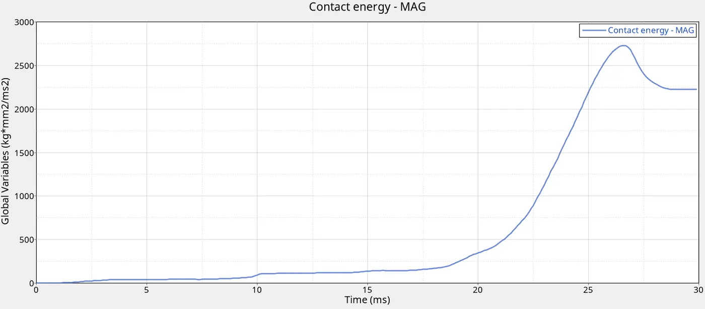
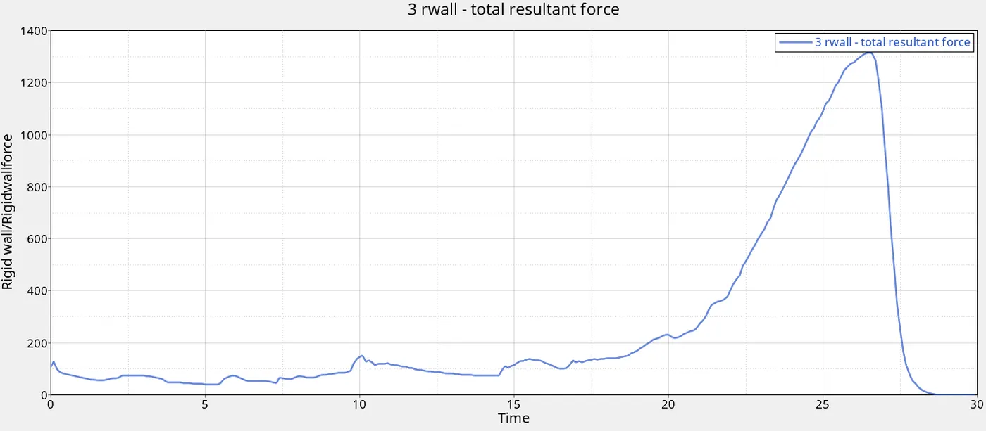
The graphs for contact energy and rigid wall forces all are similar also. They start at zero and gradually increase and reach a peak at approximately 27 ms and then drop again.

From the tabulated results, we can see that values for maximum displacement does not vary much between the cases.

Whereas, energy error percentage increases when new method of contact is added that is type 11 contact is added to the system which is changing the energy error. This can indicate that adding the new contact type might have introduced some penetrations which need to be repelled leading to energy errors. This energy error was reduced in case 4 when the notches were removed. This could indicate that the energy error increase in case 3 might have been due to the presence of the notches. Similarly in case 6 the energy error is higher than in case 5. The main change is the addition of a notch in case 6 which could further be proof that presence of notch is creating energy errors.

Addition of new contact type also could be leading to the increase in simulation time. Contact type 7 was solely used in case 1 and case 2. The rest of the cases included contact type 11 which all are having time much higher than the first two cases. This means that addition of type 11 contact although will have more accurate results comes at the cost of computational resources.Therefore , a suitable trade-off must be implemented when using these simulations in industry.

Maximum stress value also decreases significantly from cases 1 and 2 to case 3. This could mean that cases 1 and 2 which were using only type 7 contact were inaccurate with respect to stress calculation which was corrected in case 3. This stress was reduced in case 4 where the notch is removed. This means that the presence of notch can lead to stress concentration at the notch which could lead to increase in maximum stress value. This observation also is seen in cases 5 and 6 where addition of notch is leading to higher stress values.

Maximum contact force and rigid wall force both were significantly larger in case 3 when compared to cases 1 and 2. This could also be due to addition of contact type 11.

CONCLUSION: The bumper model was successfully meshed using 2D shell and 1D spot welds. The crush tubes were simulated for all 6 cases as required by the assignment. The results were tabulated, plotted and compared. Discussions were made on the observations of the results.