Assignment 4-RADIOSS Material Laws Challenge

COMPARE ALL DIFFERENT CASES WITH DIFFERENT MATERIAL LAW'S

OBJECTIVE:

Compare all the seven cases with different material law's we further study the effect in the change of Failure card and to tabulate Number of cycles, Energy error, Mass error and Simulation time for all the seven cases we performed

PROCEDURE:

• CASE 1: Import starter file
• Run the Failure_Johnson000.rad
• Explaining Recommended properties
• Check the results
• Plot the graphs
• CASE 2: Import starter file and Edit the failure card properties
• Check the results
• Plot the graphs
• CASE 3: Import starter file and Delete failure card
• Check the results
• Plot the graphs
• CASE 4: Import starter file
• Edit material property as EPS_P_max as zero
• Check the results
• Plot the graphs
• CASE 5: Import starter file
• Change the material property as M2_plast_john to M1_Elastic
• Check the results
• Plot the graphs
• CASE 6: Import starter file
• Change the material property as M2_plast_john to M36_PLAS_TAB
• Create a curve
• Check the results
• Plot the graphs
• CASE 7: Import starter file
• Run the Law27_000.rad
• Enter Recommended properties
• Check the results
• Plot the graphs

CASE 1: IMPORT STARTER FILE:

Go to Files in task bar >> Import >> Solver Deck >> FAILURE_JOHN_0000.rad (select) >> Import

The starter file stores information about:

• Nodes
• Load Conditions
• Velocity
• Boundary Conditions, etc.
• Basically, it is an ASCII (American Standard Code for Information Interchange) file that contains the model information.
• The starter file should always end with 0000.rad.

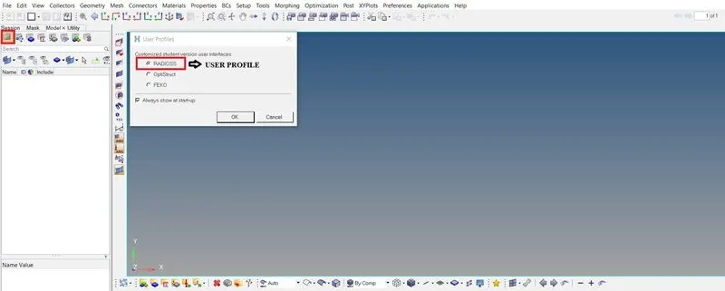
USER PROFILE

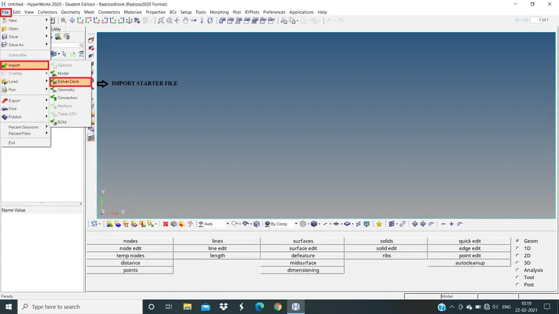
IMPORT STARTER FILE

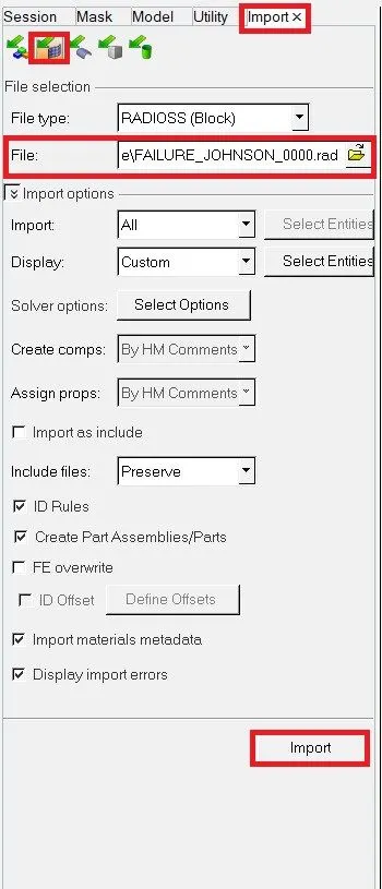
SELECT FILE

Now click to import

RECOMMENDED PROPERTIES:

Parameters		Comment
Ishell =24		QEPH 4 nodes shells are best combination of cost and accuracy.
Ismstr=2		Full geometric nonlinearities (default)with possible small strain formulation activation in RADIOSS Engine.
Ish3n=2		Standard 3 noded shell (C0) with modification for large rotation(default)
N=5		Number of integration points set to 5 for accuracy bending.
Ithick=1		Thickness change is taken into account for accuracy.
Iplas=1		Iterative plasticity for good accuracy.

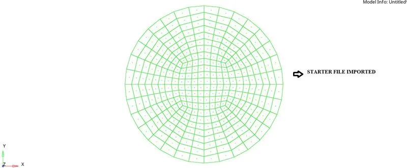
MODEL IMPORTED

After importing the model RUN the file

For that

Go to Analyize >> Radioss >> Save as >> Select file >> Radioss

Once the simulation done

Note down No. of cycle, Energy error, Mass error and Simulation time

The input file is the same Started file that we had just Edited.

Once we hit Radioss, a pop-up box will appear. It shows us the real time analysis and gives us the final result.

After run the file will contain animation video along with animation steps and time history file will be saved in the same folder where the starter file exists.

ANALYSIS PAGE

SELECT STARTER FILE

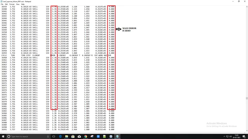
ENGINE OUT FILE

Edit the Engine File:

The engine File stores information about:

Simulation Runtime

Simulation Speed control parameters, such as No. of Animation Files, No. of Time History File, Size of the history file and Animation frequency, etc.

Basically, it is an ASCII (American Standard Code for Information Interchange) file that describes the run controls.

We can also edit the Engine File directly through the Control Cards.

Now open the animation

For that

Go to Hyperveiw >> Select animation file >> Apply

To see von-mises

Go to contour in hyperveiw >> Select von-mises >> Select: Simple >> Apply

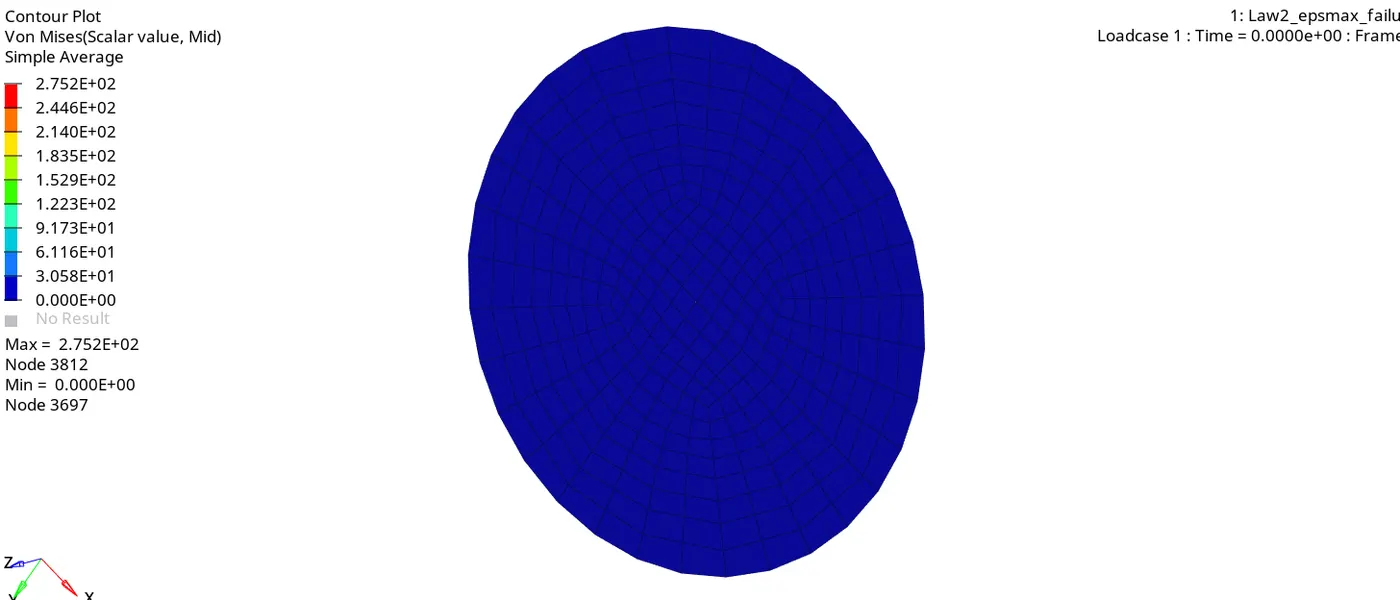
ANIMATION

After checking animation file we have to plot the graphs

For that

Go to Hyper graph 2D >> Select T01(Time history file) >> Select x-type = Time >> Y-type = Global variable >> Y-request = Internal, kinetic, contact, Hour glass and Total energies >> MAG(Magnitude) >> Apply

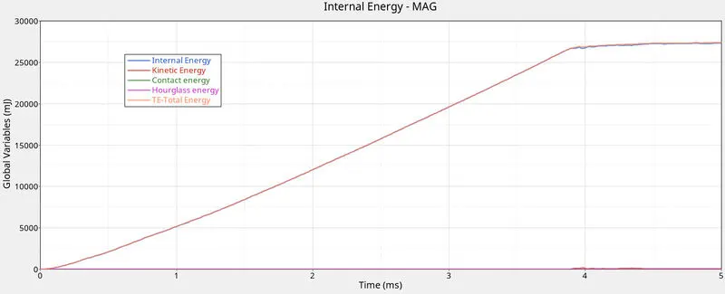
PLOTTED GRAPH

INTERNAL ENERGY:

X-axis Min = 0 Max = 5

Y-axis Min = 0 Max = 27322.44

Internal energy i.e Strain energy due to deformation increases linearly up to plastic failure and remains almost constant after.

KINETIC ENERGY:

X-axis Min = 0 Max = 5

Y-axis Min = 0 Max = 179.25

Sudden rise during the failure indicating the rate of deformation i.e displacement subjected to a velocity.

CONTACT ENERGY:

X-axis Min = 0 Max = 5

Y-axis Min = 0 Max = 0

There are no contact forces between the components so, the line is straight.

HOURGLASS ENERGY:

X-axis Min = 0 Max = 5

Y-axis Min = 0 Max = 0

There is zero hourglass energy present due to QEPH reduced integration method.

TOTAL ENERGY:

X-axis Min = 0 Max = 5

Y-axis Min = 0 Max = 27375.92

The Total energy Curve is almost similar to the Internal energy i,e Kinetic Energy is very small indicating no Energy Error

CASE 2: Import starter file and Edit the failure card properties:

Go to Analyize >> Radioss >> Save as >> Select file >> Radioss

Rename as Law2_epsmax_crack

NOTE: Make sure always we have to import given failure_johnson 000.rad file

Import given file and make changes in failure card

Go to failure card >> I fail_sh =1 >> Dadv = 1 >> IXfem = 1

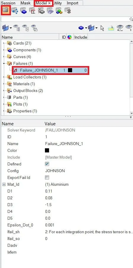
FAILURE CARD

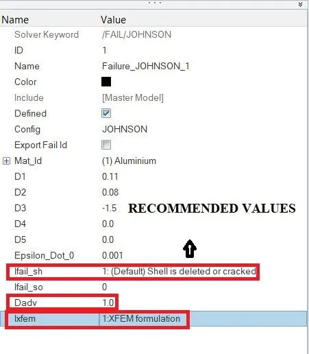
VALUES CHANGED

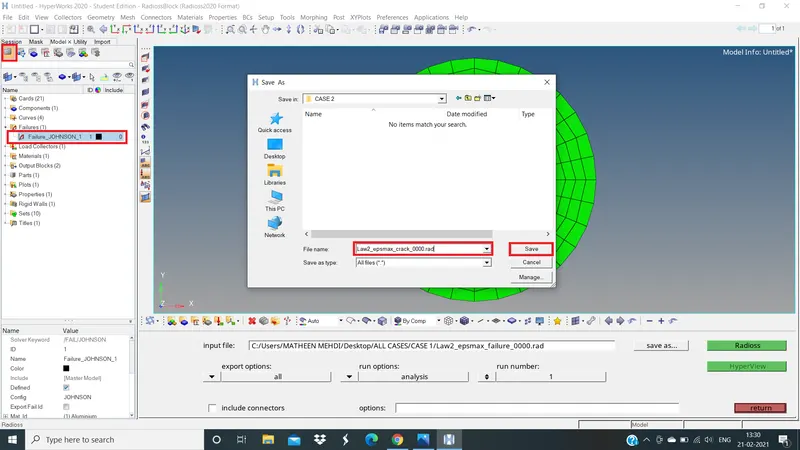
SAVE THE FILE

Now RUN the simulation

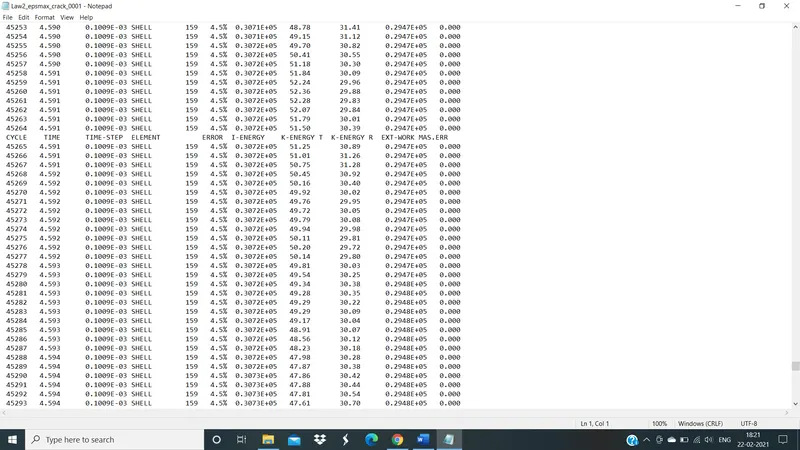
ENGINE OUT FILE

Now open the animation

For that

Go to Hyperveiw >> Select animation file >> Apply

To see von-mises

Go to contour in hyperveiw >> Select von-mises >> Select: Simple >> Apply

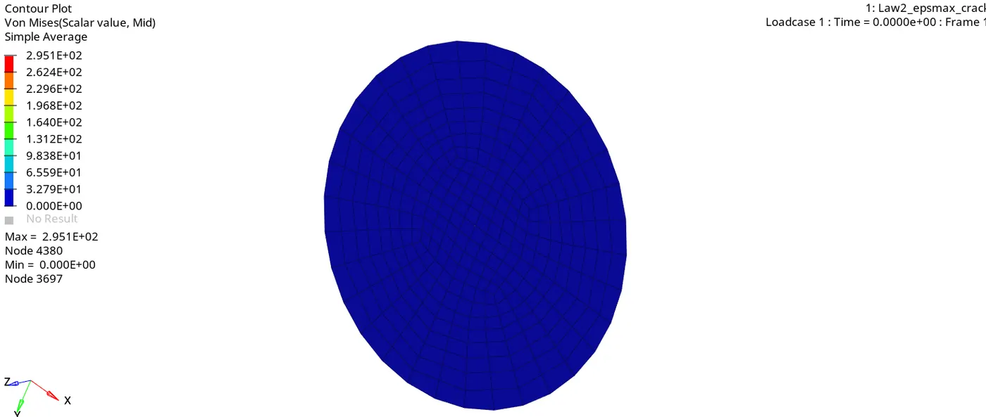
ANIMATION

After checking animation file we have to plot the graphs

For that

Go to Hyper graph 2D >> Select T01(Time history file) >> Select x-type = Time >> Y-type = Global variable >> Y-request = Internal, kinetic, contact, Hour glass and Total energies >> MAG(Magnitude) >> Apply

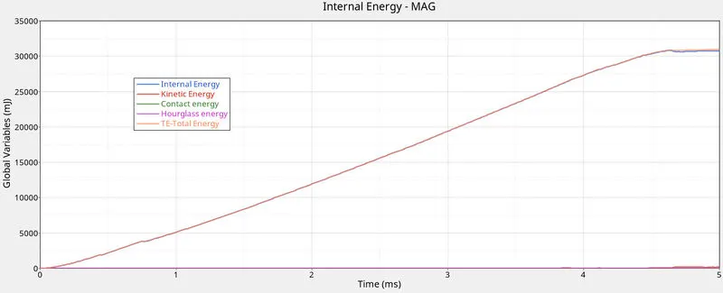
GRAPH PLOTTED

INTERNAL ENERGY:

X-axis Min = 0 Max = 5

Y-axis Min = 0 Max = 27322.44

Internal energy i.e Strain energy due to deformation increases linearly up to plastic failure and remains almost constant afterwards.

KINETIC ENERGY:

X-axis Min = 0 Max = 5

Y-axis Min = 0 Max = 179.25

Increases rapidly compare to case 1. The rate of deformation is controlled by the Johnson Failure parameters.

CONTACT ENERGY:

X-axis Min = 0 Max = 5

Y-axis Min = 0 Max = 0

There are no contact forces between the components so, the line is straight.

HOURGLASS ENERGY:

X-axis Min = 0 Max = 5

Y-axis Min = 0 Max = 0

There is zero hourglass energy present due to QEPH reduced integration method.

TOTAL ENERGY:

X-axis Min = 0 Max = 5

Y-axis Min = 0 Max = 27375.92

The Total energy Curve is almost similar to the Internal energy i,e Kinetic Energy is very small indicating no Energy Error

CASE 3: Import starter file and Delete failure card:

Go to Analyize >> Radioss >> Save as >> Select file >> Radioss

Rename as Law2_epsmax_nofail

NOTE: Make sure always we have to import given failure_johnson 000.rad file

Import given file and make chnages in failure card

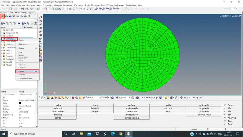
DELETE FAILURE CARD

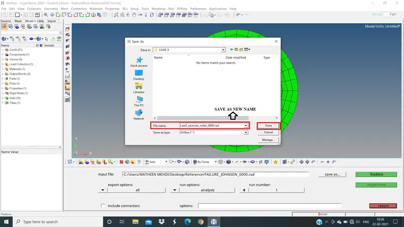
RENAME AS LAW2_EPSMAX_NOFAIL

Now RUN the simulation

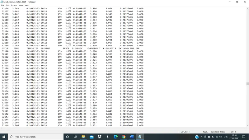
ENGINE OUT FILE

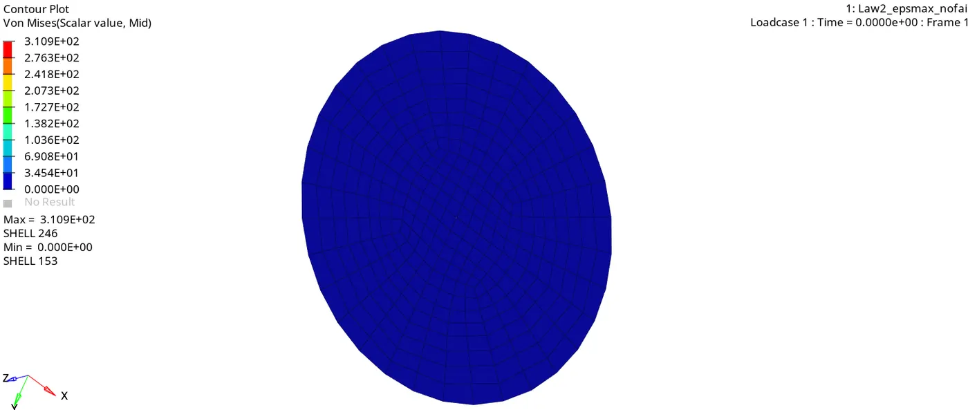
Now open the animation

For that

Go to Hyperveiw >> Select animation file >> Apply

To see von-mises

Go to contour in hyperveiw >> Select von-mises >> Select: Simple >> Apply

ANIMATION

After checking animation file we have to plot the graphs

For that

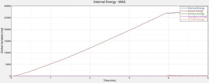
Go to Hyper graph 2D >> Select T01(Time history file) >> Select x-type = Time >> Y-type = Global variable >> Y-request = Internal, kinetic, contact, Hour glass and Total energies >> MAG(Magnitude) >> Apply

GRAPH PLOTTED

INETRNAL ENERGY:

X-axis Min = 0 Max = 5

Y-axis Min = 0 Max = 27443.066

Internal energy i.e Strain energy due to deformation increases linearly up to plastic failure and remains almost constant after.

KINETIC ENERGY:

X-axis Min = 0 Max = 5

Y-axis Min = 0 Max = 332.07

As there is no failure criteria, maximum deformation occurs i.e displacement subjected to a velocity leading to a rise during the failure.

CONTACT ENERGY:

X-axis Min = 0 Max = 5

Y-axis Min = 0 Max = 0

There are no contact forces between the components so, the line is straight.

HOURGLASS ENERGY:

X-axis Min = 0 Max = 5

Y-axis Min = 0 Max = 0

There is zero hourglass energy present due to QEPH reduced integration method.

TOTAL ENERGY:

X-axis Min = 0 Max = 5

Y-axis Min = 0 Max = 27528.36

The Total energy Curve is almost similar to the Internal energy i,e Kinetic Energy is very small indicating no Energy Error

CASE 4: Import starter file and change the EPS_max value as zero:

Go to Analyize >> Radioss >> Save as >> Select file >> Radioss

Rename as Law2_EPS_P_max

NOTE: Make sure always we have to import given failure_johnson 000.rad file

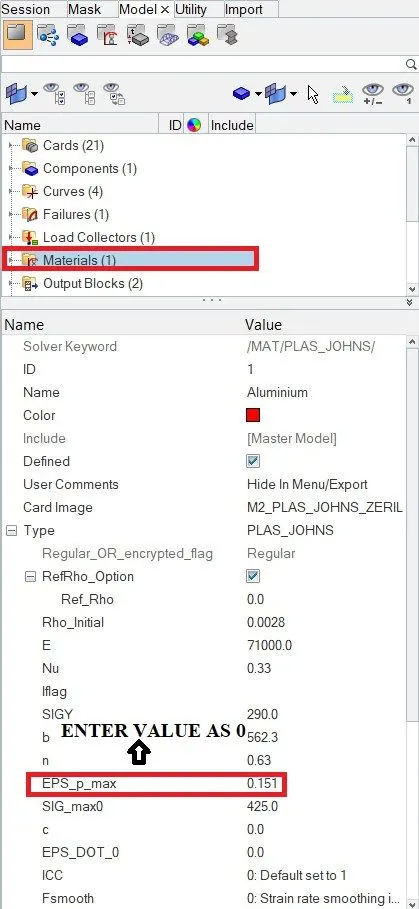
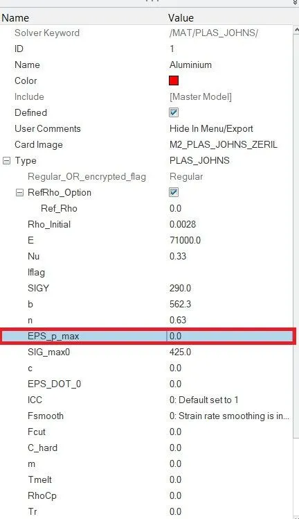
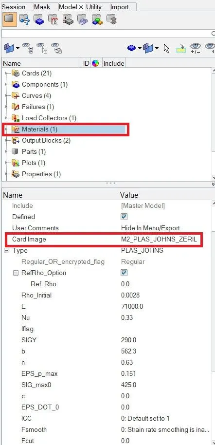
Import given file and make changes in material card

Set EPS_p_max as zero

MATERIAL CARD

SET AS EPS_p_max AS ZERO

Now RUN the simulation

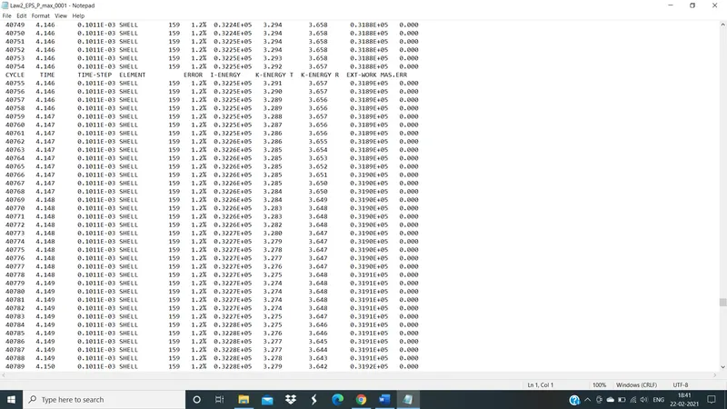
ENGINE OUT FILE

Now open the animation

For that

Go to Hyperveiw >> Select animation file >> Apply

To see von-mises

Go to contour in hyperveiw >> Select von-mises >> Select: Simple >> Apply

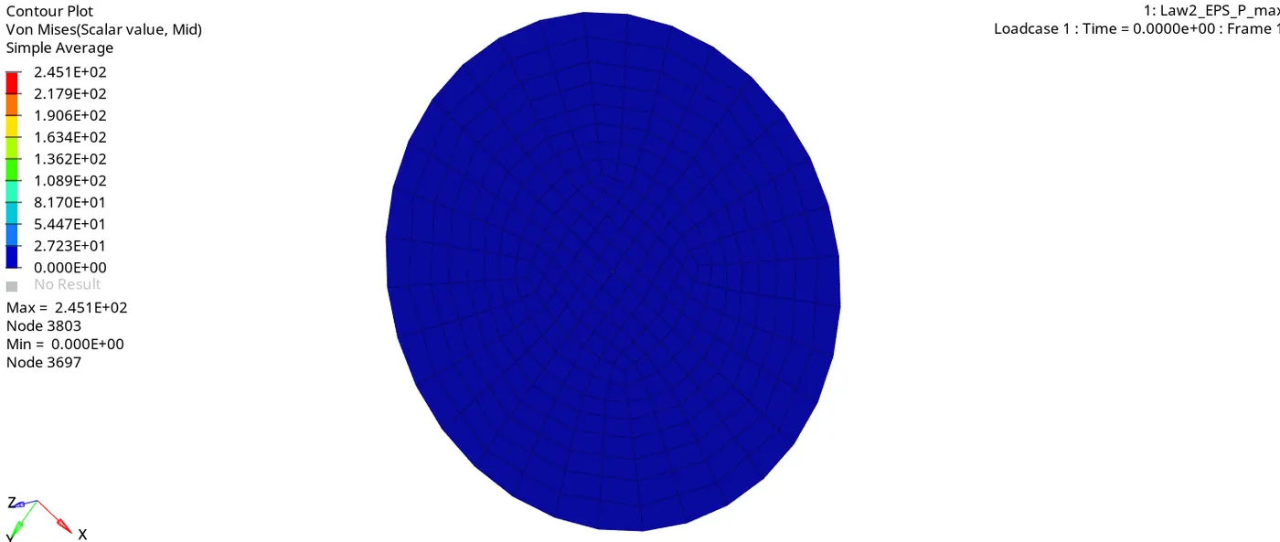
ANIMATION

After checking animation file we have to plot the graphs

For that

Go to Hyper graph 2D >> Select T01(Time history file) >> Select x-type = Time >> Y-type = Global variable >> Y-request = Internal, kinetic, contact, Hour glass and Total energies >> MAG(Magnitude) >> Apply

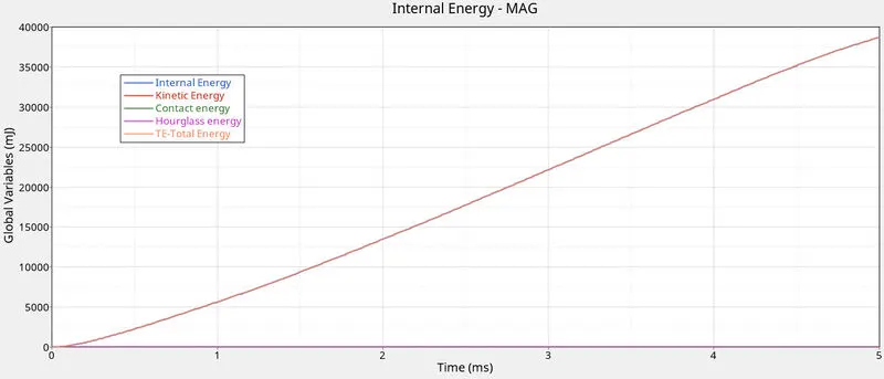
GRAPH PLOTTED

INETRNAL ENERGY:

X-axis Min = 0 Max = 5

Y-axis Min = 0 Max = 38724.82

The Strain energy continues to increase at the same rate even after cracking is initiated. This result is undesirable and no material possess infinite strain rate.

KINETIC ENERGY:

X-axis Min = 0 Max = 5

Y-axis Min = 0 Max = 15.23

The element is bending at a very low rate so the Kinetic energy produced on the element is also less due to slow rate of deformation.

CONTACT ENERGY:

X-axis Min = 0 Max = 5

Y-axis Min = 0 Max = 0

There are no contact forces between the components so, the line is straight.

HOURGLASS ENERGY:

X-axis Min = 0 Max = 5

Y-axis Min = 0 Max = 0

There is zero hourglass energy present due to QEPH reduced integration method.

TOTAL ENERGY:

X-axis Min = 0 Max = 5

Y-axis Min = 0 Max = 38728.76

The Total energy Curve is almost similar to the Internal energy i,e Kinetic Energy is very small indicating no Energy Error

CASE 5: Import starter file and change the material card :

Go to material card change M2_plas_john_zeril to M1_Elastic

Go to Analyize >> Radioss >> Save as >> Select file >> Radioss

Rename as Law1_Ealstic

NOTE: Make sure always we have to import given failure_johnson 000.rad file

Import given file and make changes in material card

MATERIAL CARD

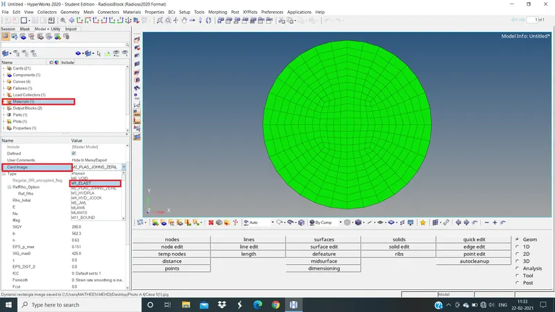
CHANGED TO LAW1

After changing enter value

E = 71000

NU = 0.33

Rho_initial = 0.0028

Now RUN the simulation

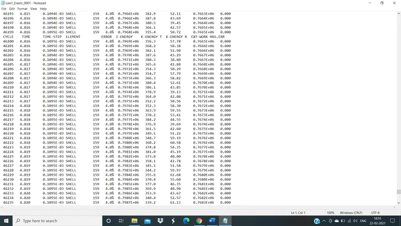
ENGINE OUT FILE

Now open the animation

For that

Go to Hyperveiw >> Select animation file >> Apply

To see von-mises

Go to contour in hyperveiw >> Select von-mises >> Select: Simple >> Apply

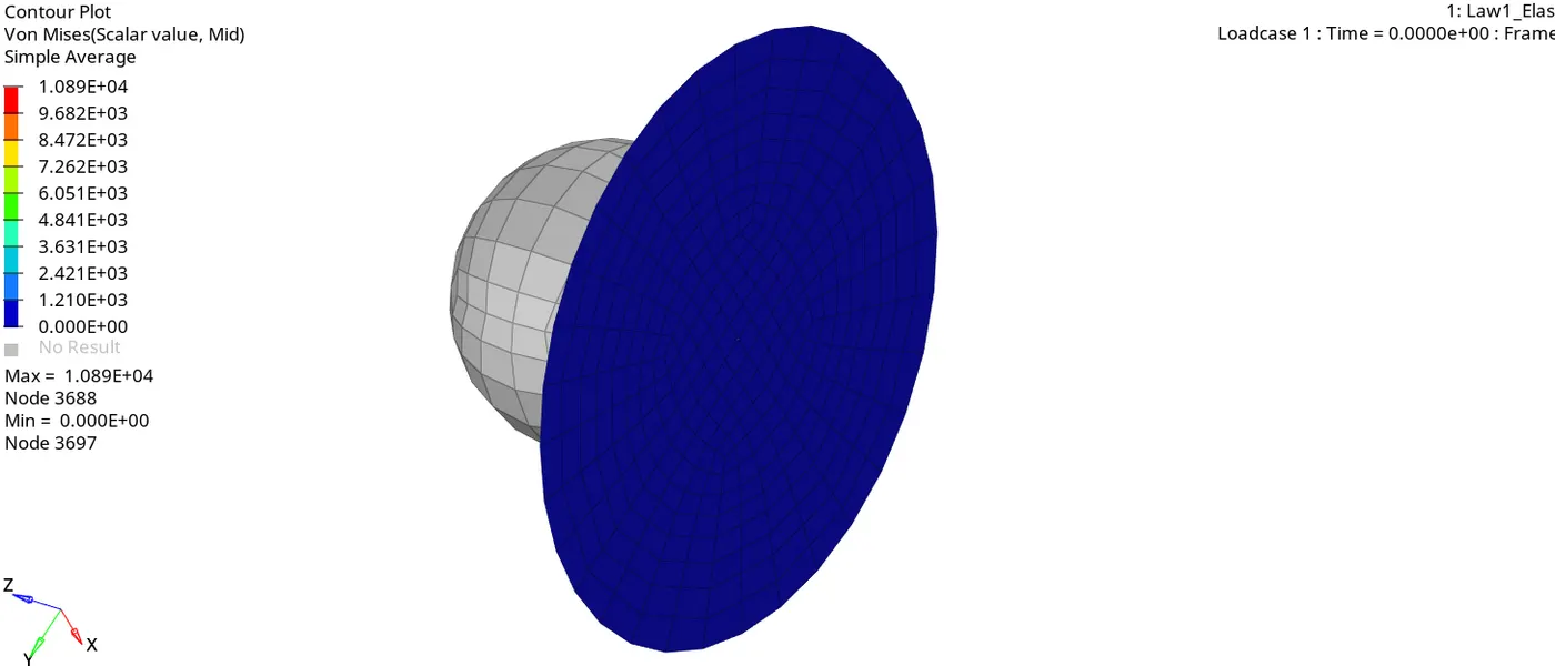
ANIMATION

After checking animation file we have to plot the graphs

For that

Go to Hyper graph 2D >> Select T01(Time history file) >> Select x-type = Time >> Y-type = Global vairiable >> Y-request = Internal, kinetic, contact, Hour glass and Total energies >> MAG(Magnitude) >> Apply

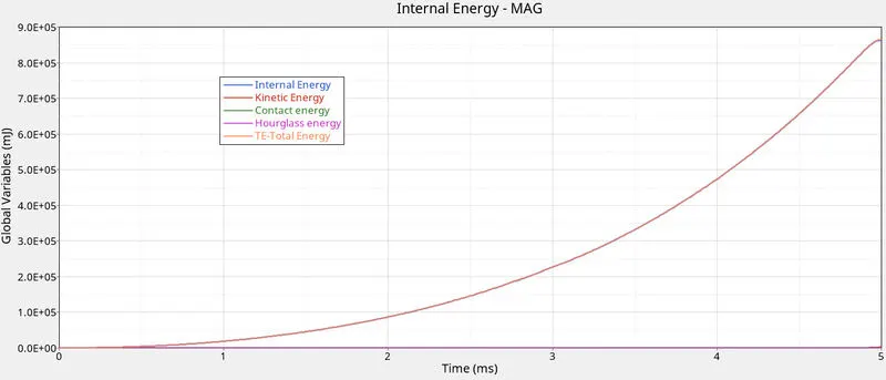
GRAPH PLOTTED

INETRNAL ENERGY:

X-axis Min = 0 Max = 5

Y-axis Min = 0 Max = 862533.37

Internal energy i.e Strain energy due to deformation increases only linearly as it has an infinite elastic limit Only elasticity, no plasticity involved.

KINETIC ENERGY:

X-axis Min = 0 Max = 5

Y-axis Min = 0 Max = 3245.74

Kinetic energy almost remains constant, but increases during maximum deformation.

CONTACT ENERGY:

X-axis Min = 0 Max = 5

Y-axis Min = 0 Max = 0

There are no contact forces between the components so, the line is straight.

HOURGLASS ENERGY:

X-axis Min = 0 Max = 5

Y-axis Min = 0 Max = 0

There is zero hourglass energy present due to QEPH reduced integration method.

TOTAL ENERGY:

X-axis Min = 0 Max = 5

Y-axis Min = 0 Max = 865645.75

The Total energy Curve is almost similar to the Internal energy i,e Kinetic Energy is very small indicating no Energy Error

CASE 6: Import starter file and change the material card :

Go to material card change M2_plas_john_zeril to M36_Plas_Tab

Go to Analyize >> Radioss >> Save as >> Select file >> Radioss

Rename as LAW 36

NOTE: Make sure always we have to import given failure_johnson 000.rad file

Import given file and changes in material card

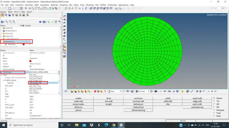
MATERIAL CARD

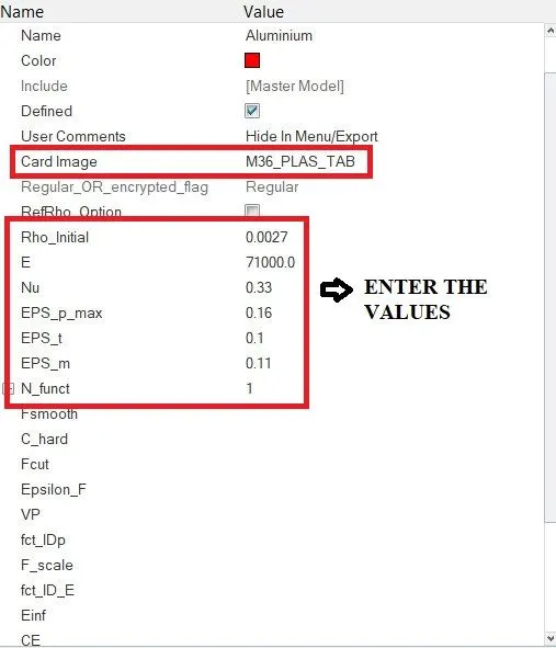
ENTER THE VALUES AS PER CHART

Now create a new curve

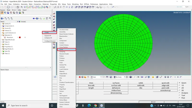
CREATING A CURVE

Curve editor box will open

Click to NEW as shown in below fig

Enter name as CASE 6 >> PROCEED

CARD image will open

Click to RETURN

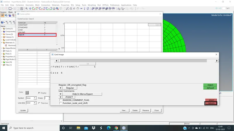
RENAME AS CASE 6

Now Edit X and Y value as per the chart

After entered the value click to update

Now we can see the graph in graphical region as shown in below fig

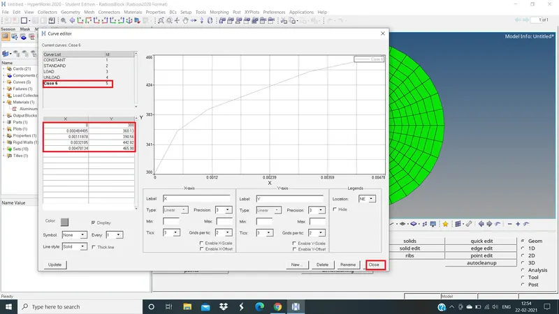
CURVE CREATED

Now go to material card >> Select N_Funt: Fct-ID(select case 6 curve ) >> Assign >> ok

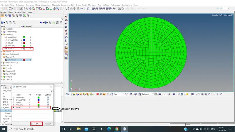
ASSIGNING CURVE

Now this changes file has to save in Law_36

Run the simulation

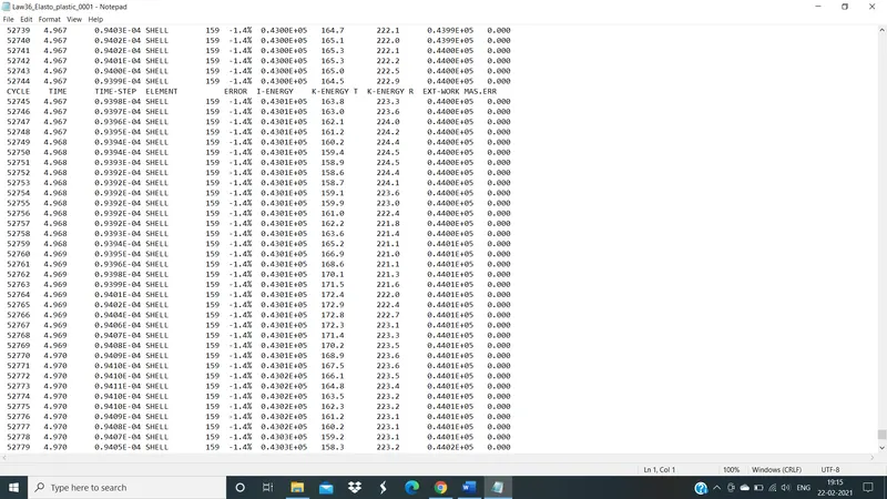
ENGINE OUT FILE

Now open the animation

For that

Go to Hyperveiw >> Select animation file >> Apply

To see von-mises

Go to contour in hyperveiw >> Select von-mises >> Select: Simple >> Apply

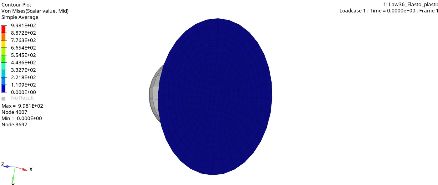
ANIMATION

After checking animation file we have to plot the graphs

For that

Go to Hyper graph 2D >> Select T01(Time history file) >> Select x-type = Time >> Y-type = Global variable >> Y-request = Internal, kinetic, contact, Hour glass and Total energies >> MAG(Magnitude) >> Apply

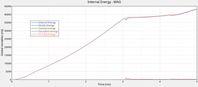
GRAPH PLOTTED

INETRNAL ENERGY:

X-axis Min = 0 Max = 5

Y-axis Min = 0 Max = 43207.44

Internal energy i.e Strain energy due to deformation increases linearly up to plastic failure and further increases slowly due to D1, D2, D3 until the element is deleted.

KINETIC ENERGY:

X-axis Min = 0 Max = 5

Y-axis Min = 0 Max = 1086.47

Rise in Kinetic energy at two points.

CONTACT ENERGY:

X-axis Min = 0 Max = 5

Y-axis Min = 0 Max = 0

There are no contact forces between the components so, the line is straight.

HOURGLASS ENERGY:

X-axis Min = 0 Max = 5

Y-axis Min = 0 Max = 0

There is zero hourglass energy present due to QEPH reduced integration method.

TOTAL ENERGY:

X-axis Min = 0 Max = 5

Y-axis Min = 0 Max = 43366.17

The Total energy Curve is almost similar to the Internal energy i,e Kinetic Energy is very small indicating no Energy Error

CASE 7: IMPORT LAW_27:

Go to Analyize >> Radioss >> Save as >> Select file >> Radioss

Rename as Law27

NOTE: Make sure always we have to import given failure_johnson 000.rad file

Import given file and enter recommended properties

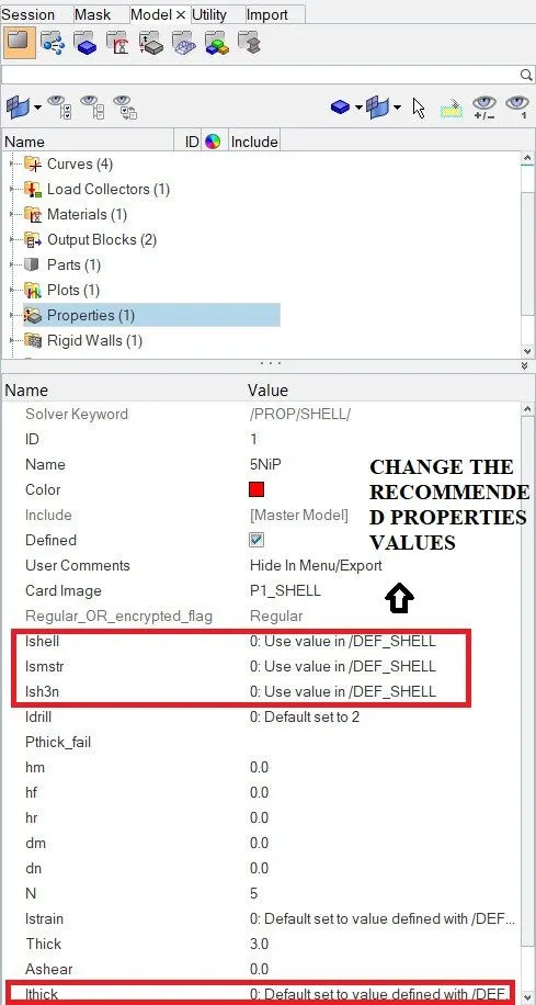
MATERIAL CARD

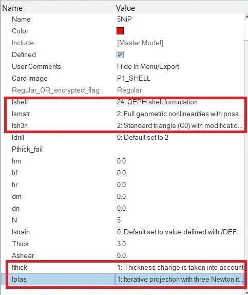
ENTERED RECOMMENDED PROPERTIES

Now RUN the simulation

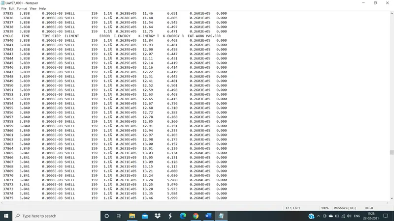
ENGINE OUT FILE

Now open the animation

For that

Go to Hyperveiw >> Select animation file >> Apply

To see von-mises

Go to contour in hyperveiw >> Select von-mises >> Select: Simple >> Apply

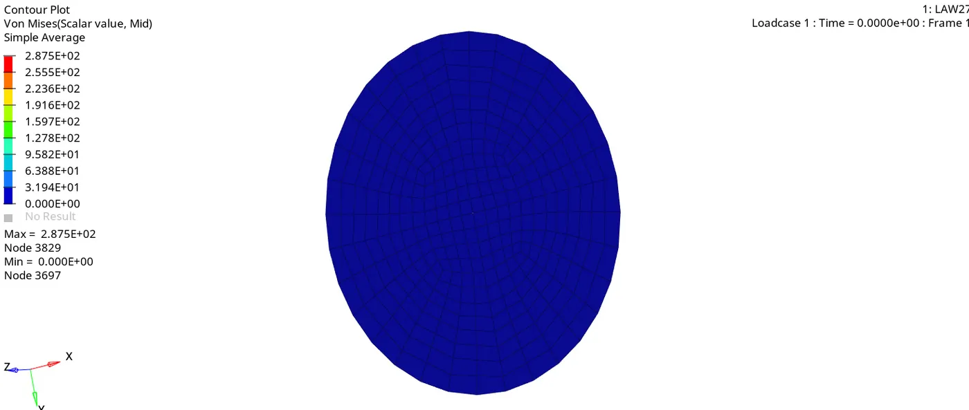
ANIMATION

After checking animation file, we have to plot the graphs

For that

Goto Hyper graph 2D >> Select T01(Time history file) >> Select x-type = Time >> Y-type = Global variable >> Y-request = Internal, kinetic, contact, Hour glass and Total energies >> MAG(Magnitude) >> Apply

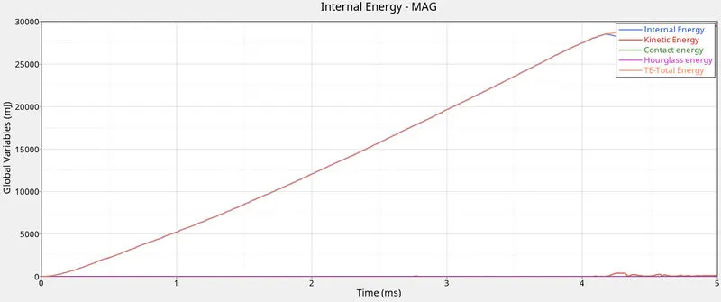
GRAPH PLOTTED

INETRNAL ENERGY:

X-axis Min = 0 Max = 5

Y-axis Min = 0 Max = 29476.73

Since Brittle, the strength is very high leading to a higher yield point.

KINETIC ENERGY:

X-axis Min = 0 Max = 5

Y-axis Min = 0 Max = 425.88

At different stages of penetration on the plate, the elements are failing quickly and there are many rises in the energy curve caused by the deformation i.e displacement subjected to a velocity.

CONTACT ENERGY:

X-axis Min = 0 Max = 5

Y-axis Min = 0 Max = 0

There are no contact forces between the components so, the line is straight.

HOURGLASS ENERGY:

X-axis Min = 0 Max = 5

Y-axis Min = 0 Max = 0

There is zero hourglass energy present due to QEPH reduced integration method.

TOTAL ENERGY:

X-axis Min = 0 Max = 5

Y-axis Min = 0 Max = 29581.28

The Total energy Curve is almost similar to the Internal energy i,e Kinetic Energy is very small indicating no Energy Error

Case No.	Current Law	Change to Law	Changes in the Material Parameters	Description
1	Law 2		Run as it is	EPSmax & σmaxσmax are the failure criterias. They are Ultimate Stress and Strain values from the Stress strain curve.
2	Law 2		Change the failure parameters in Johnson Failure Card: Ifail_sh = 1 Dadv = 1 Ixfem = 1	D1, D2 & D3 (from Strain rate data) are the failure criteria's.
3	Law 2		Delete the /Fail/JOHNSON Material Card	Failure criteria's
4	Law 2		Delete EPS_p_max	When EPS_p_max is set to zero, we get Infinite Strain. Simulation will stop element reaches σmax
5	Law 2	Law 1	Keep the Density, Young's Modulus, and Poisson's ratio same as that in Law 2 material card	Material is completely Elastic, i.e. Infinite strain rate. There are no Failure criteria's, therefore the elements won't fail.
6	Law 2	LAW36	The elastic region is defined by Density, Young's Modulus, and Poisson's Ratio. The plastic region is defined by the rupture parameters.	The Rupture parameters are : EPS_t : Strain at the beginning of Tensile Damage EPS_m : Strain at the end of Tensile Damage Epsilon_F : Tensile Failure Strain [The above are rupture parameters for Torsion only] EPS_p_max : Plastic Failure Strain [The last one is a combined failure]
7	Law 27			The failure parameters are: et: strain at the beginning of Tensile Failure em: Maximum Tensile strain dmax: Maximum Damage factor ef: Max. Tensile strain for Element deletion

These are all the changes we have done as per the given question

Comparing all the 7 cases as per the tabulated Number of cycles, Energy error, Mass error and Simulation time shows in below table

Cases	Total number of cycles	Energy Error	Mass Error	Total Simulation Time in S
1	49379	-0.6% to 1.3%	0.00%	114.48
2	49216	-0.6% to 4.6%	0.00%	128.88
3	49407	-0.6% to 1.2%	0.00%	109.43
4	49303	-0.6% to 1.2%	0.00%	111.89
5	47968	-0.6% to 4.0%	0.00%	105.80
6	53200	-1.4% to 0.6%	0.00%	120.87
7	49506	-0.6% to 1.1%	0.00%	39.70

CONCLUSION:

Based on the stress and strain conditions given Law 36 is more suitable as it follows the results of real time testing and shows the behaviour of a real-world material i.e elasticity and plasticity and I would like to conclude that this assignment helped me to understand how to see the material behaviour and how to change the material law's and how to plot the required graphs and how to study them.