Assignment 4-RADIOSS Material Laws Challenge

RADIOSS Material Laws Challenge

Objective:

To perform simulation as per the cases given below.

CASE 1: To run a simulation using given FAILURE_JOHNSON_0000.rad file and rename it as Law2_epsmax_failure.

CASE 2: To run a simulation using Case 1, Law2_epsmax_failure file and rename it as Law2_epsmax_crack.

Changes to be made in /FAIL/JOHNSON card for Case 2 simulation.

• ifail_sh = 1
• Dadv = 1
• Ixfem = 1

CASE 3: To run a simulation using Case 2, Law2_epsmax_crack file and rename it as Law2_epsmax_nofail.

Simulation to be done by removing the fail_Johnson failure card

CASE 4: To run a simulation using Case 3, Law2_epsmax_nofail file

Simulation to be done by removing both the failure plastic strain (EPS_p_max) and the fail_Jhonson failure card.

CASE 5: To run a simulation using Case 4.

Simulation to be done by changing the material card to Law 1.

CASE 6: To run a simulation using Case 1, Law2_epsmax_failure file.

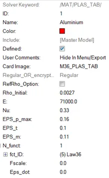
Simulation to be done with the law 36 material card.

CASE 7: To run a simulation using given Law27_0000.rad file

Simulation to be done with the law 27 material card.

Then compare all the 7 Cases based on

• Total number of cycles, Energy error, mass error, and simulation time.
• Notice the animation of all 5 and describe the animations in brief based on whether the elements are being deleted or cracked.
• Plot energies and notice any difference.
• Based on all the results, which case would represent the on-field scenario.
• Prepare a ppt/Docx and list down case by case results and your conclusion as to why the failure happened.

Procedures:

Case 1:

The given FAILURE_JOHNSON_0000.rad file is imported to hyperworks and shaded elems view is displayed in Figure 1.

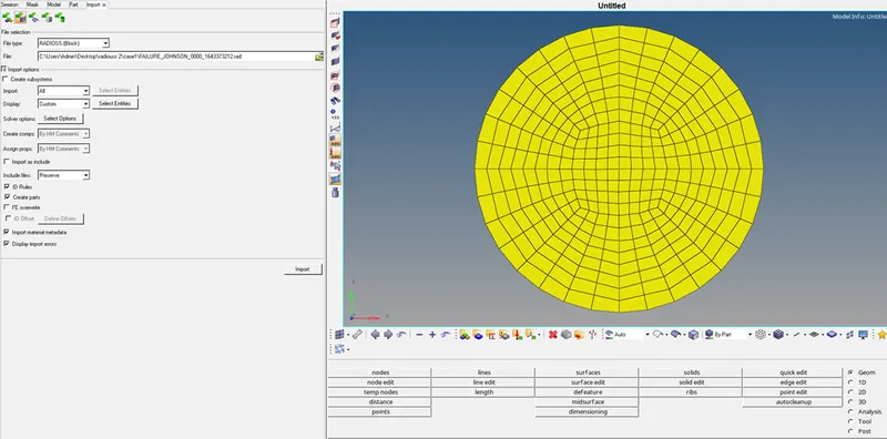
Figure 1: Imported rad file

Then check Standard units using the begin card as shown in figure 2. As per Case 1, this simulation is performed with the default values as shown in figure 3, 4 & 5.

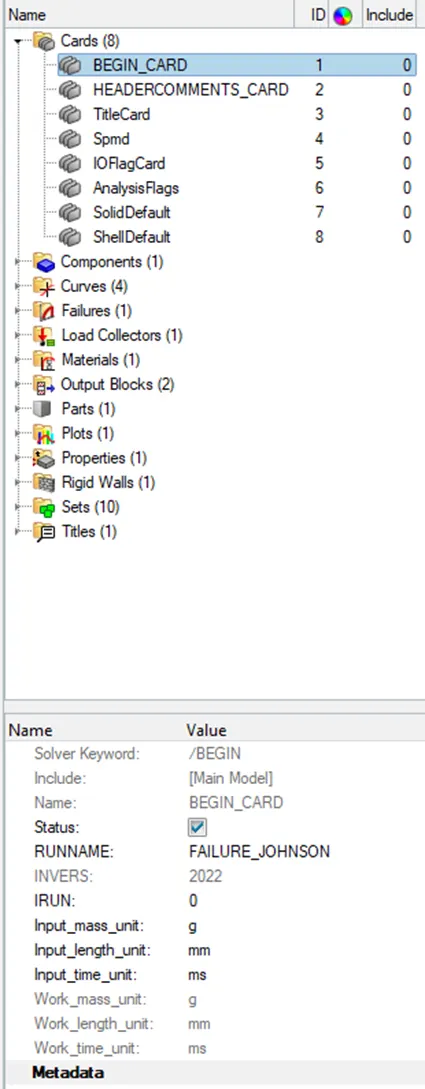
Figure 2: Begin card

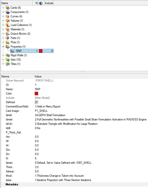
Figure 3: Properties Card

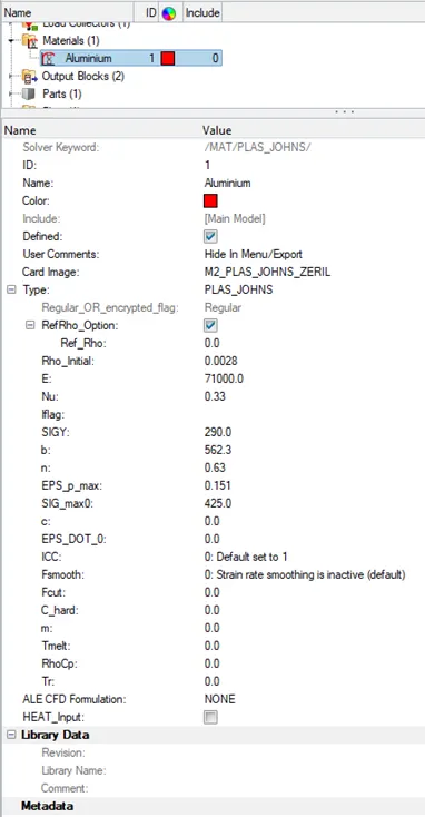
Figure 4: Materials Card

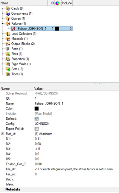
Figure 5: Failure Card

To run simulation >> ANALYSIS+RADIOSS and in that options panel assign as -nt 4 as shown in Figure 6. This refers to assigning the work to the system's four cores which will speed up the simulation, while "nt" stands for "number of threads." then select "Radioss" to launch the simulation. it will show RADIOSS JOB IS COMPLETED in Console solver view tab as displayed in Figure 7.

Figure 6: RADIOSS analysis panel

Click on RESULT in that tab, it will direct to hyperview where the animation of the simulation is viewed. Animation file are in name of h3d will be in the load area in this panel then switch to contour mode in the panel and assign the result type as Von Mises(s) with scalar value and click apply.

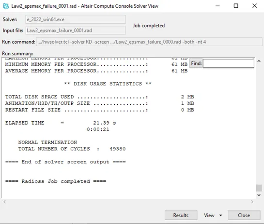
Figure 7: Console solver view tab

Result of Von Mises (s) case 1 simulation and the animation of the simulation in hyperview is shown as in figure 8.

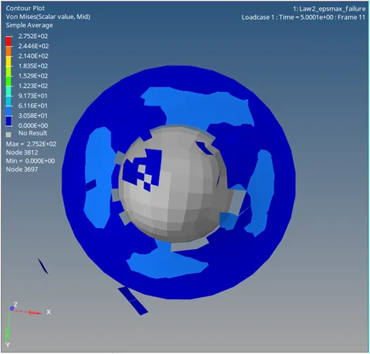
Figure 8: Case 1,Von Mises (s) simulation results

Open output of simulation in 0001.out file which is generated after the simulation. The final energy error is 0.8 percentage, which lies in between the safe tolerance percentage as shown in Figure 9. i.e,safe tolerance percentage = -15% TO +5%

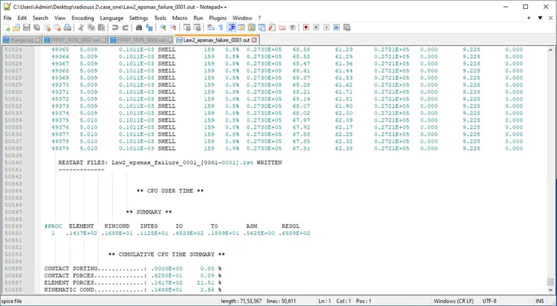
Figure 9: 0001.out file of Case 1.

Case 2:

Same procedure of Case 1 is performed along the change in Failure card as shown in Figure 10.

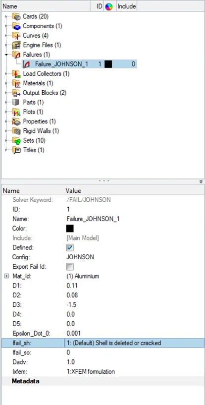
Figure 10: Case 2, Failure Card

Arrived Console solver view tab for Case 2 is as displayed in Figure 11.

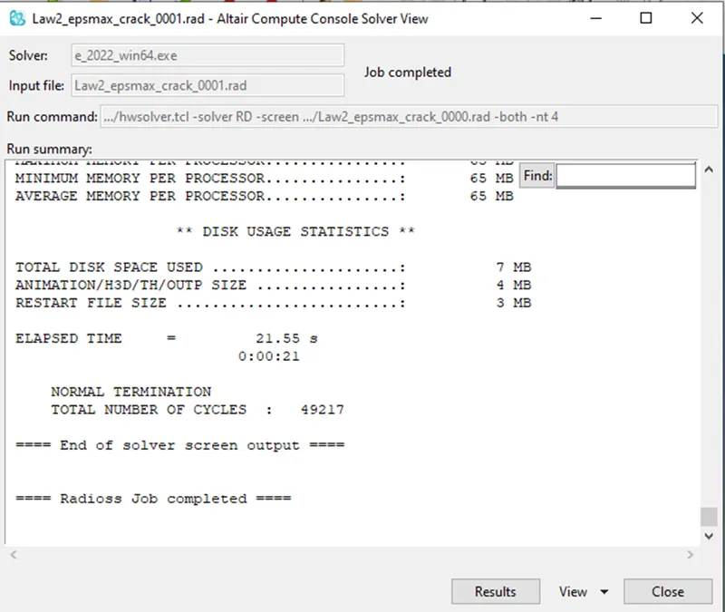
Figure 11: Case 2, Console solver view tab

Result of Von Mises (s) case 2 simulation and the animation of the simulation in hyperview is shown as in Figure 12.

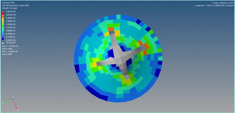
Figure 12: Case 2, Von Mises (s) simulation results

Open output of simulation in 0001.out file which is generated after the Case 2 simulation. The final energy error is 4.1 percentage, which lies in between the safe tolerance percentage as shown in Figure 13.

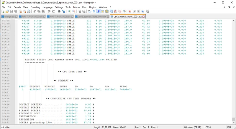
Figure 13: 0001.out file of Case 2.

Case 3:

Same procedure of Case 2 is performed along with removing the fail_Johnson failure card as shown in Figure 14.

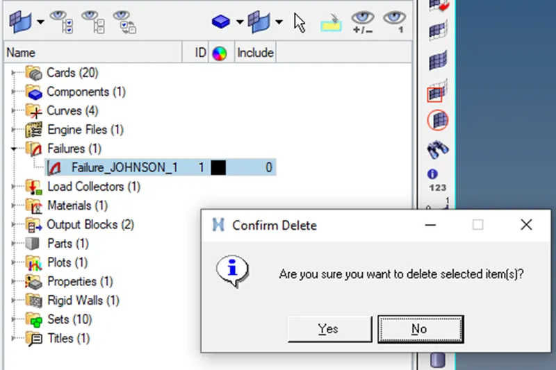
Figure 14: Removing Failure Card

Arrived Console solver view tab for Case 3 is as displayed in Figure 15.

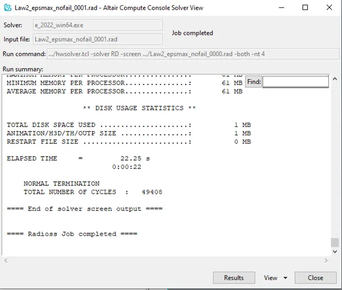
Figure 15: Case 3, Console solver view tab

Result of Von Mises (s) Case 3 simulation and the animation of the simulation in hyperview is shown as in Figure 16.

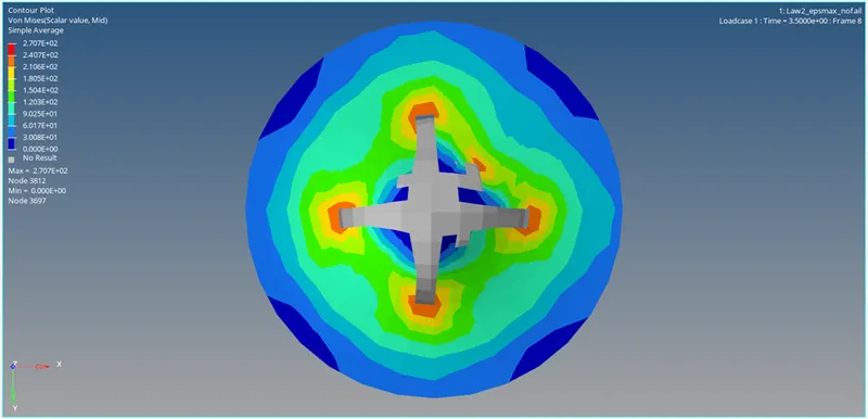
Figure 16: Case 3, Von Mises (s) simulation results

Open output of simulation in 0001.out file which is generated after the Case 3 simulation. The final energy error is 0.8 percentage, which lies in between the safe tolerance percentage as shown in Figure 17.

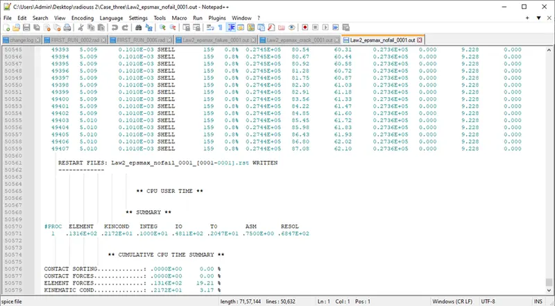
Figure 17: 0001.out file of Case 3.

Case 4:

Same procedure of Case 3 is performed along with removing failure plastic strain (EPS_p_max) as a add on with fail_Johnson failure card as shown in Figure 18

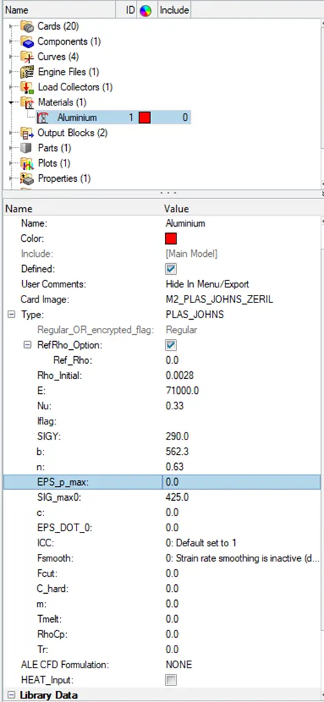
Figure 18: Material card (removing EPS_p_max)

Arrived Console solver view tab for Case 4 is as displayed in Figure 19.

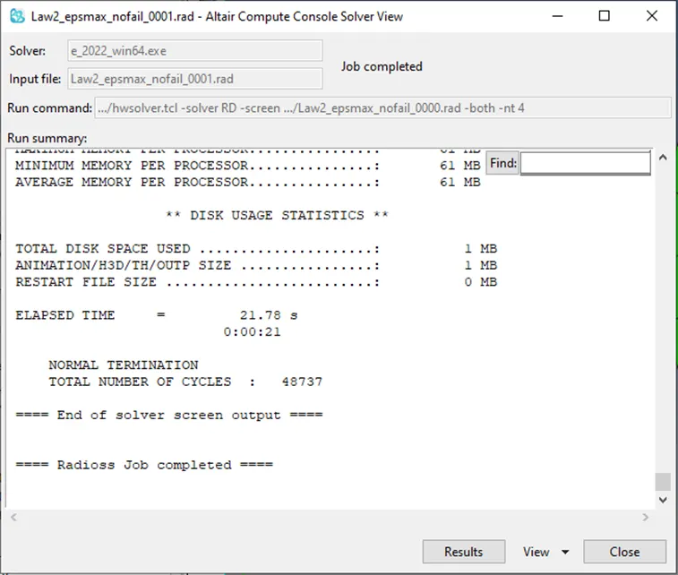
Figure 19: Console solver view tab, Case 4.

Result of Von Mises (s) Case 4 simulation and the animation of the simulation in hyperview is shown as in Figure 20.

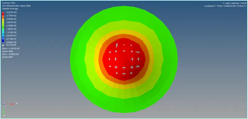
Figure 20: Case 4, Von Mises (s) simulation results

Open output of simulation in 0001.out file which is generated after the Case 4 simulation. The final energy error is 3.0 percentage, which lies in between the safe tolerance percentage as shown in Figure 21.

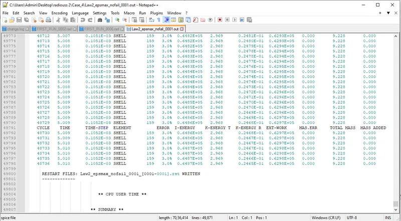
Figure 21: 0001.out file of Case 4.

Case 5:

Same procedure of Case 3 is performed along with change in the material card to Law 1 as shown in Figure 22.

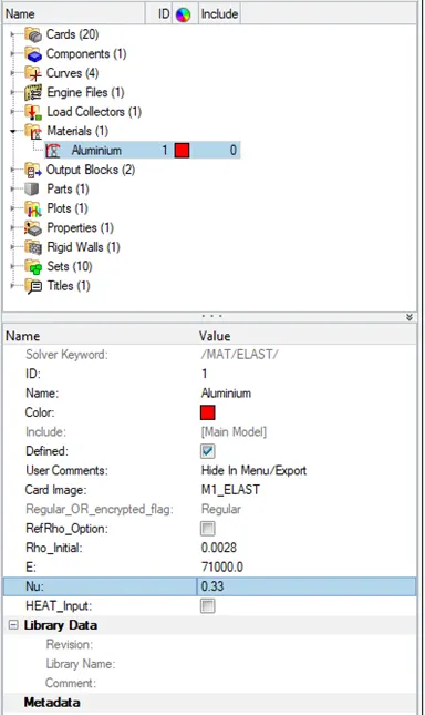
Figure 22: Case 5, Material Card.

Arrived Console solver view tab for Case 5 is as displayed in Figure 23.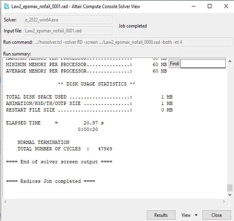

Figure 23: Console solver view tab, Case 5.

Result of Von Mises (s) Case 5 simulation and the animation of the simulation in hyperview is shown as in Figure 24.

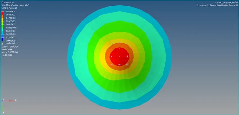
Figure 24: Case 5, Von Mises (s) simulation results

Open output of simulation in 0001.out file which is generated after the Case 5 simulation. The final energy error is 1.3 percentage, which lies in between the safe tolerance percentage as shown in Figure 25.

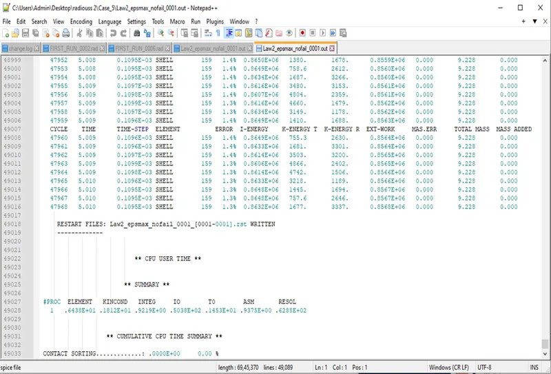
Figure 25: 0001.out file of Case 5.

Case 6:

Same procedure of Case 1 is performed along the change in the material card to Law 36. Law 36 is a isotropic elasto-plastic material which consists of an model N_funct curve panel, which to be assigned using user-defined functions (curve). The Created curve is shown in Figure 26. The created curve is applied to the Law 36 material card as shown in Figure 27.

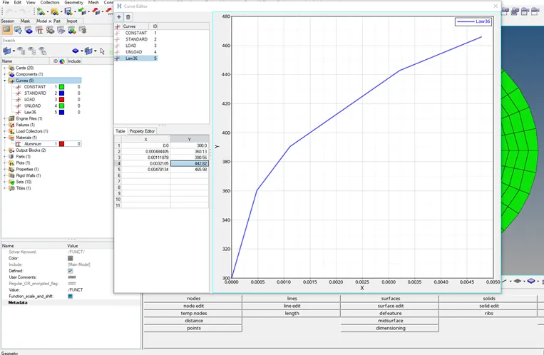
Figure 26: Created Law 36 curve.

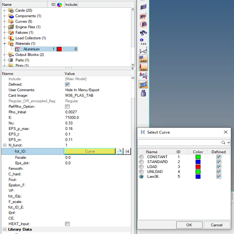
Figure 27: fct_ID assigning in Material Card

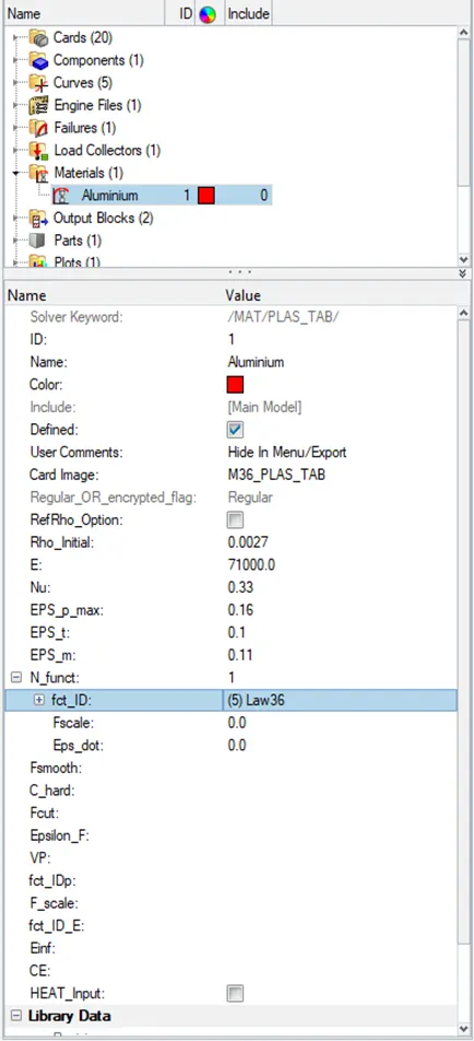
Figure 28: Required Material Card

Arrived Console solver view tab for Case 6 is as displayed in Figure 29.

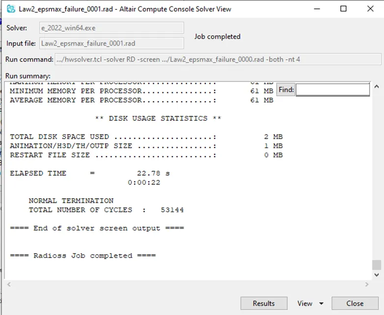
Figure 29: Console solver view tab, Case 6.

Result of Von Mises (s) Case 6 simulation and the animation of the simulation in hyperview is shown as in Figure 30.

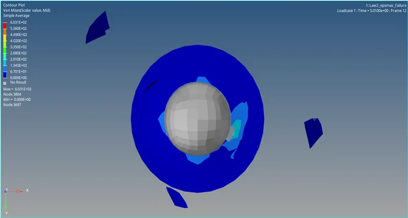
Figure 30: Case 6, Von Mises (s) simulation results

Open output of simulation in 0001.out file which is generated after the Case 5 simulation. The final energy error is -1.8 percentage, which lies in between the safe tolerance percentage as shown in Figure 31.

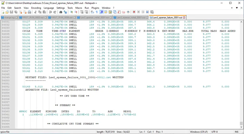
Figure 31: 0001.out file of Case 6.

Case 7:

The given Law27_0000.rad file is imported and the simulation is performed with the Law 27 material card with recommended shell properties as shown in Figure 32.

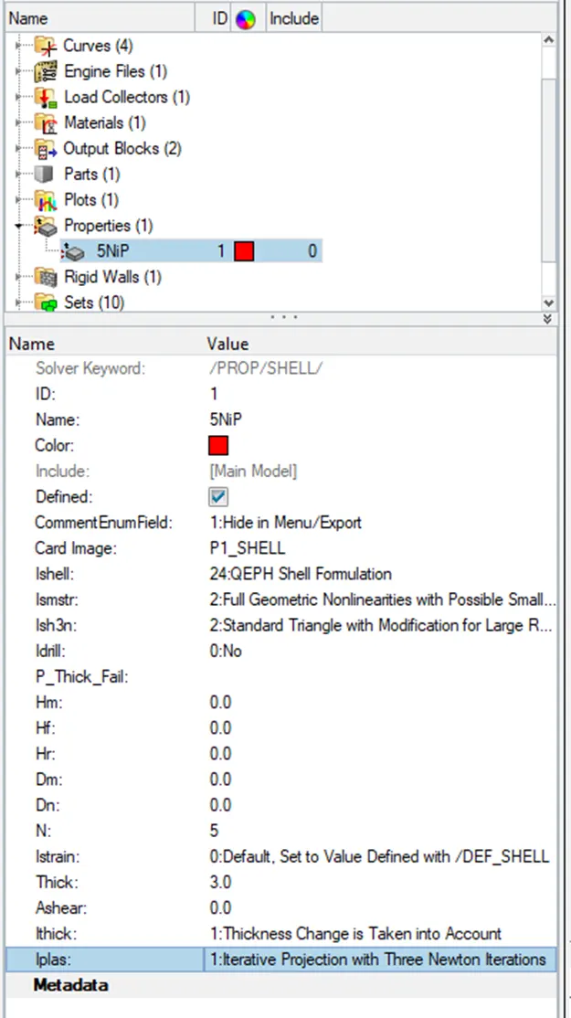
Figure 32: Law 27 Material Card

Arrived Console solver view tab for Case 7 is as displayed in Figure 33.

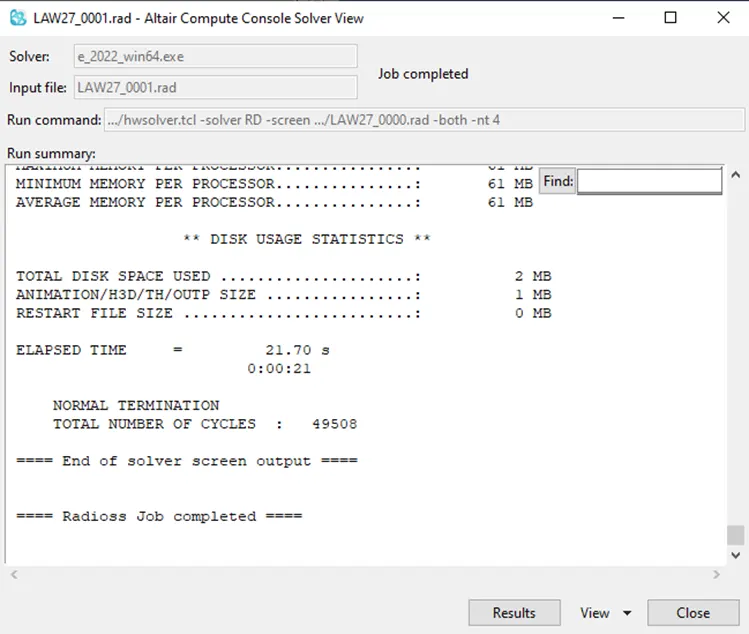
Figure 33: 0001.out file of Case 7.

Result of Von Mises (s) Case 7 simulation and the animation of the simulation in hyperview is shown as in Figure 34.

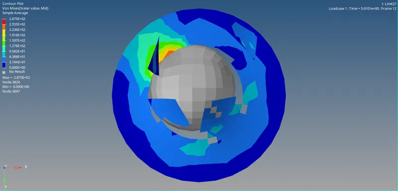
Figure 34: Case 7, Von Mises (s) simulation results

Open output of simulation in 0001.out file which is generated after the Case 7 simulation. The final energy error is 0.8 percentage, which lies in between the safe tolerance percentage as shown in Figure 35.

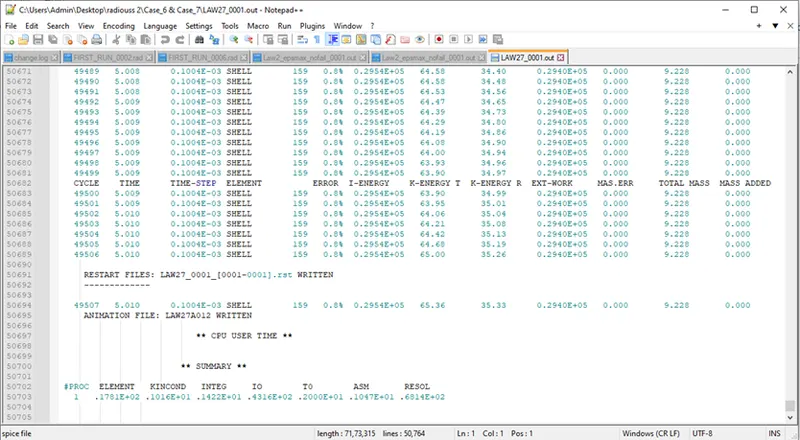
Figure 35: 0001.out file of Case 7.

Graph:

Case 1

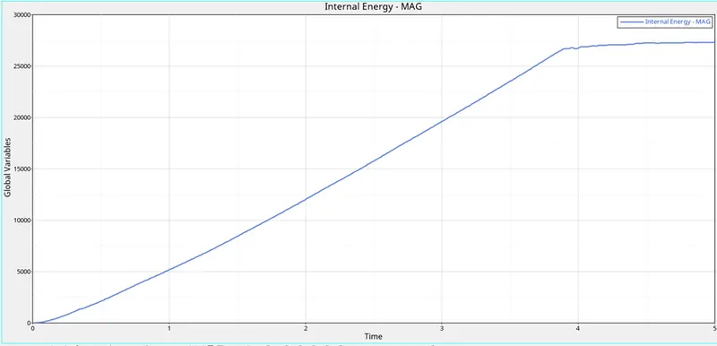
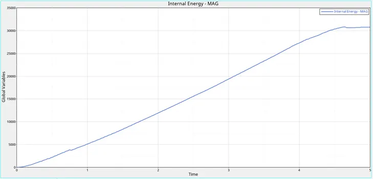
Internal energy

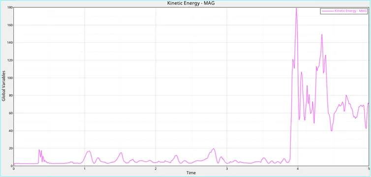
Kinetic energy

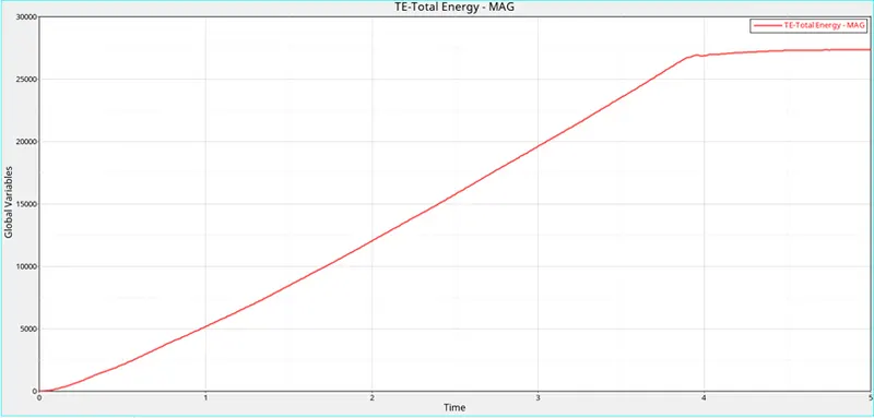
Total Energy

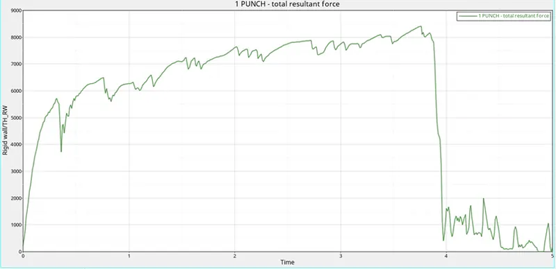
Total Resultant force

Case 2

Internal energy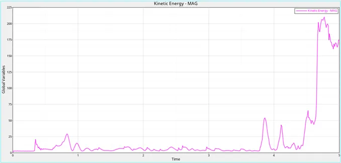

Kinetic energy

Total Energy

Total Resultant force

Case 3

Internal energy

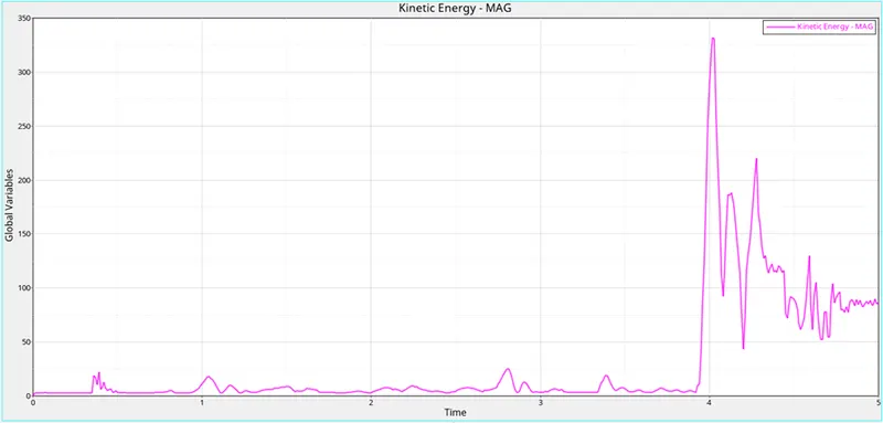
Kinetic energy

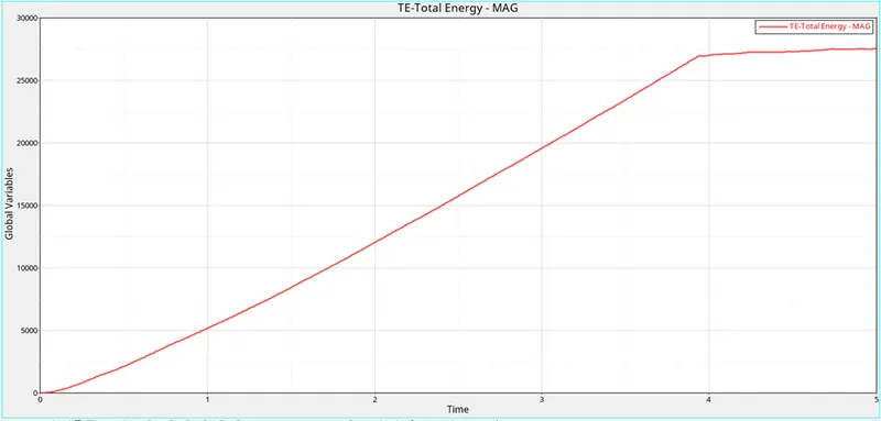
Total Energy

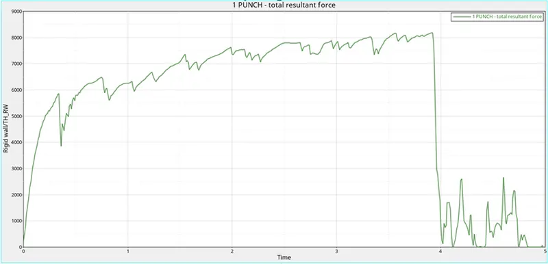
Total Resultant force

Case 4

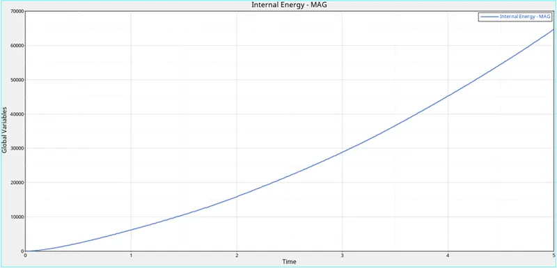
Internal energy

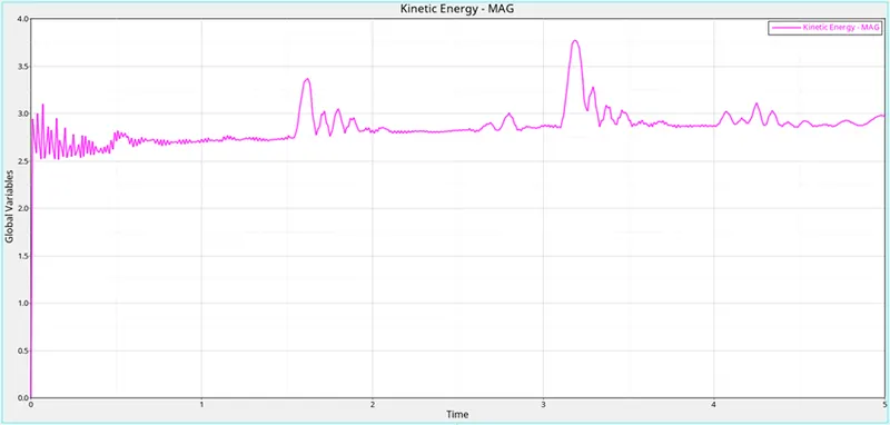
Kinetic energy

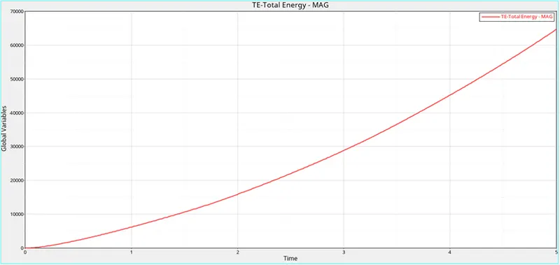
Total Energy

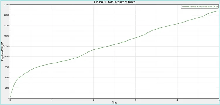
Total Resultant force

Case 5

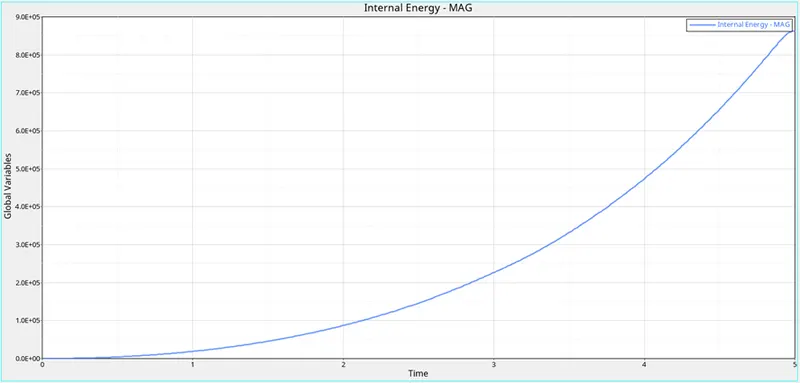
Internal energy

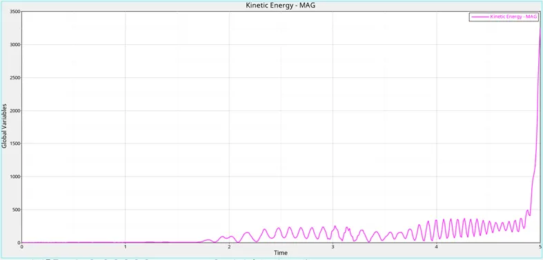
Kinetic energy

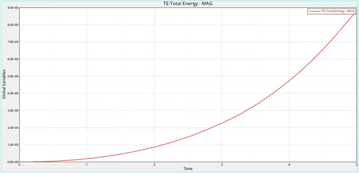
Total Energy

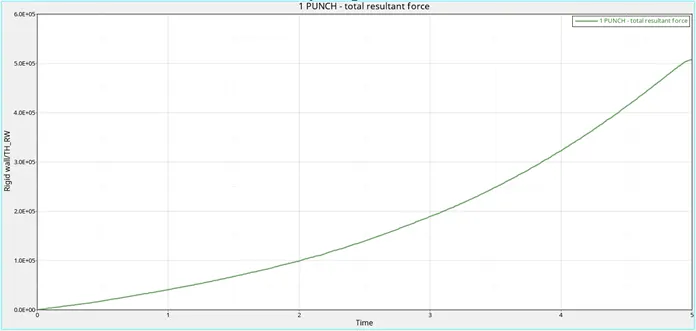
Total Resultant force

Case 6

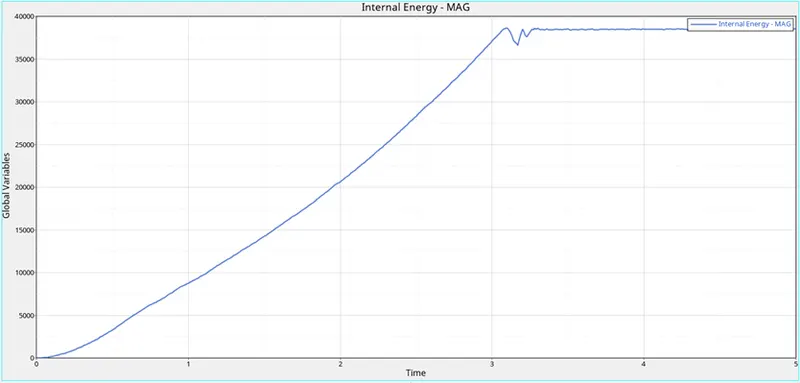
Internal energy

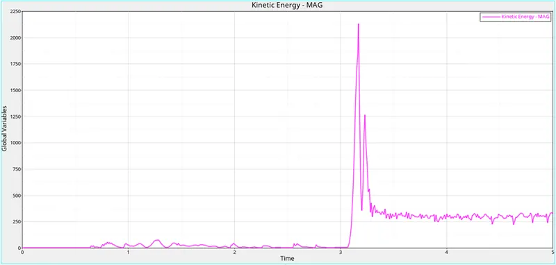
Kinetic energy

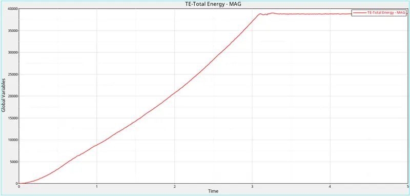
Total Energy

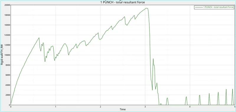
Total Resultant force

Case 7

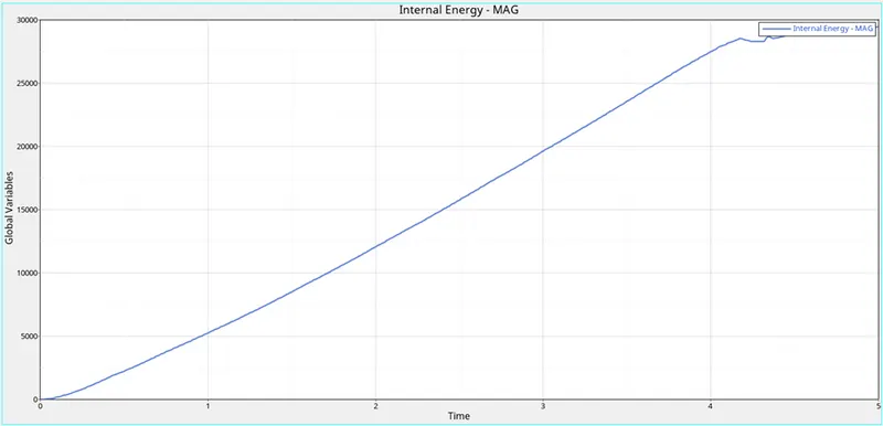
Internal energy

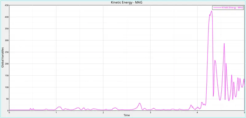
Kinetic energy

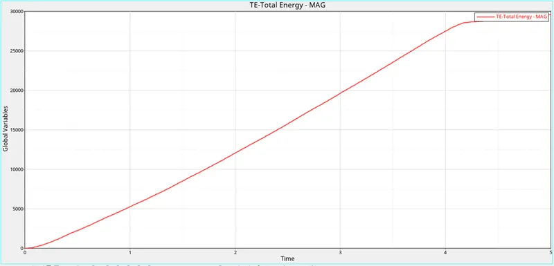
Total Energy

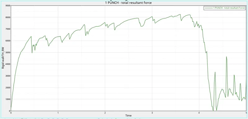
Total Resultant force

Comparison

	CASE 1	CASE 2	CASE 3	CASE 4
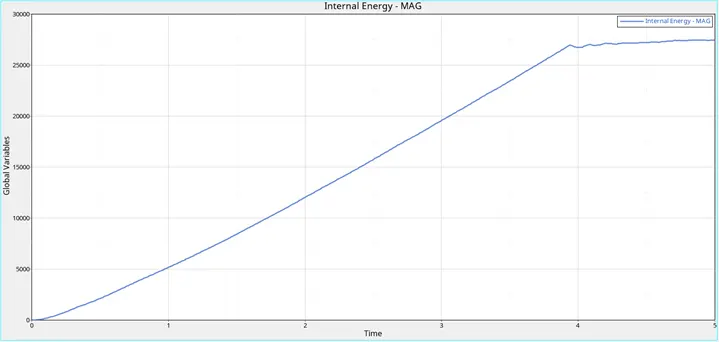
Internal energy	Internal energy, Rises from the initial point from origin and reaches steadily between of 25000 to 3000 global variable with time step between 3 to 4 then maintained steadily.	Internal energy, Rises from the initial point from origin and reaches steadily between of 30000 to 3500 global variable with time step between 4 to 5 then maintained steadily.	Internal energy, Rises from the initial point from origin and reaches steadily between of 25000 to 3000 global variable with time step between 3 to 4 then maintained steadily.	Internal energy, Rises from the initial point from origin and reaches steadily between of 60000 to 7000 global variable with time step between 4 to 5 then maintained steadily.
Kinetic energy	The peak of Kinetic energy, attains at 4 time step with global variable 180. then fluctuate after that maximum peak	The peak of Kinetic energy, attains between 4 and 5 time step with global variable 200 to 225. then fluctuate after that maximum peak	The peak of Kinetic energy, attains between 4 and 5 time step with global variable 300 to 350. then fluctuate after that maximum peak	Kinetic energy Rises at the initial point which is origin up to 3.0 global variable and steadily fluctuate to a maximum peak between 3.5 to 4.0 global variable with time step in between 3 to 4.
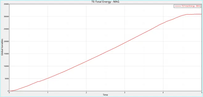
Total energy	Total energy, Rises from the initial point from origin and reaches steadily between of 25000 to 3000 global variable with time step between 3 to 4 then maintained steadily.	Total energy, Rises from the initial point from origin and reaches steadily between of 30000 to 3500 global variable with time step between 4 to 5 then maintained steadily.	Total energy, Rises from the initial point from origin and reaches steadily between of 25000 to 3000 global variable with time step between 3 to 4 then maintained steadily.	Total Energy, Rises from the initial point from origin and reaches steadily between of 60000 to 7000 global variable with time step between 4 to 5 then maintained steadily.
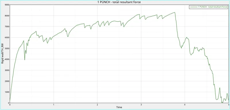
Total resultant force	Total resultant Force, attains the maximum peak between of 8000 to 9000 global variable with time step between 3 to 4 then fluctuate after that maximum peak .	Total resultant Force, attains the maximum peak between of 8000 to 9000 global variable with time step between 3 to 4 then fluctuate after that maximum peak .	Total resultant Force, attains the maximum peak between of 8000 to 9000 global variable with time step between 3 to 4 then fluctuate after that maximum peak .	Total resultant Force, attains the maximum peak between of 2000 to 2250 global variable with time step between 4 to 5 then fluctuate after that maximum peak .
	CASE 5	CASE 6	CASE 7
Internal energy	Internal energy, Rises from the initial point from origin and reaches steadily between of 80E+05 to 90E+05 global variable with time step between 4 to 5 then maintained steadily.	Internal energy, Rises from the initial point from origin and reaches steadily between of 35000 to 40000 global variable with time step between 3 to 4 then fluctuate slightly then maintained steadily.	Internal energy, Rises from the initial point from origin and reaches steadily between of 25000 to 30000 global variable with time step between 4 to 5 then maintained steadily.
Kinetic energy	Kinetic energy Rises from the initial point which is origin and fluctuate with in 0 to 500 global variable upto 4.7 time step and reaches a maximum peak between 3000 to3500 global variable at 5 time step.	The peak of Kinetic energy, attains between 3 and 4 time step with global variable 2000 to 2250. then fluctuate after that maximum peak	The peak of Kinetic energy, attains between 4 and 5 time step with global variable 400 to 450. then fluctuate after that maximum peak
Total energy	Total energy Rises from the initial point from origin and reaches steadily between of 80E+05 to 90E+05 global variable with time step between 4 to 5 then maintained steadily.	Total energy, Rises from the initial point from origin and reaches steadily between of 35000 to 40000 global variable with time step between 3 to 4 then fluctuate slightly then maintained steadily.	Total energy, Rises from the initial point from origin and reaches steadily between of 25000 to 30000 global variable with time step between 4 to 5 then maintained steadily.
Total resultant force	Rises from the initial point from origin and reaches steadily slightly above 50E+05 global variable with time step between 4 to 5 then maintained steadily.	Total resultant Force, attains the maximum peak between of 18000 to 20000 global variable with time step between 3 to 4 then fluctuate after that maximum peak	Total resultant Force, attains the maximum peak between of 8000 to 9000 global variable with time step between 3 to 4 then fluctuate after that maximum peak

CONCLUSION:

From Graph comparison

• From all the graph plots it clearly shows the given time step is reflected accurately in the results.
• From Internal energy plot of all 7 Cases shows that maximum peak attained at between 3 to 5 time steps and maintained a steady flat curve after attaining the peak in all plots, its reveals the stability of the internal energy in all the cases.
• From Total energy plot of all 7 Cases shows similar plots of respective Internal energy plots, hence the internal energy has the maximum part in the total energy of the analysis.
• From Kinetic energy plot of all 7 Cases shows that the maximum peak attained at between 3 to 5 time steps , it shows that the maximum kinetic energy is attained at the mid and final stages of all analysis.
• As a irony kinetic energy is heightened in the initial stage of Case 4 (but not attained to the maximum peak) and minimam initial stages in all other cases, which shows that the removal of plastic and failure cards may lead to initial increment of Kinetic energy
• From Total resultant force plot of all 7 Cases shows that maximum peak attained at between 4 to 5 time steps with fluctuation and fluctuate after attaining the peak in all plots.

From Von Mises (s) simulation results

• Case 2 presents the on-field scenario when compared to the other cases, based on the stresses that were created in the material and provided material data for aluminium with a yield stress of 290MPa and a maximum stress of 425MPa.