Assignment 4-RADIOSS Material Laws Challenge

Crashworthiness Analysis using HyperMesh and Radioss

#Assignment 4-RADIOSS Material Laws Challenge

AIM: Changing materials Laws and observing 7 different cases, their animations and other parameters.

OBJECTIVES: Johnson Cook Materials

(1). Running the model as it is given in challenge, observing simulation, discussing number of cycles it takes, energy error,mass error and plotting energies graph, naming it as law2_epsmax_failure.

(2). In Fail/Johnson collector changing ifail_sh=1, dadv=1, Ixfem=1 and running the model name as law2_epsmax_crack, observing simulation, discussing number of cycles it takes, energy error and plotting energies graph.

(3). Deleting Fail/Johnson card, running the model name as law2_epsmax_nofail , observing simulation, discussing the number of cycles it takes, energy error, mass error and plotting energies graph.

(4). Deleting the value of esp_p_max_, running the model name as law2, observing simulation, discussing the number of cycles it takes, energy error, mass error and plotting energies graph.

(5). Converting the material model to law1 elastic with same density, E, Nu, observing simulation, checking the number of cycles it takes, energy error, mass error and plotting energies graph.

(6). Converting the card to law36 elasto plastic based giving data as per given in challenge, observing simulation, checking the number of cycles it takes, energy error, mass error and plotting energies graph.

(7).Opening Law27_0000.rad, changing the shell properties to recommended shell property, running that model with law27 material card, observing simulation, checking the number of cycles it takes, energy error, mass error and plotting energies graph

PROCEDURE FOR OBJECTIVE 1 :Running the model as it is given in challenge, observing simulation, discussing number of cycles it takes, energy error,mass error and plotting energies graph, naming it as law2_epsmax_failure.

STEP 1: Open Hyperworks in Radioss solver.

STEP 2: Import Solver desk FAILURE_JOHNSON_0000.rad file

STEP 3:

• Analysis>Radioss>save as input FAILURE_JOHNSON_0000.rad file
• Save path as --case1/law2_epsmax_failure_0000.rad
• Checkbox include collectors
• Write (-nt 4) in options
• Click Radioss

STEP 4: Switch to Hyper view

STEP 5: select local model and result law2_epsmax_failure.h3d file

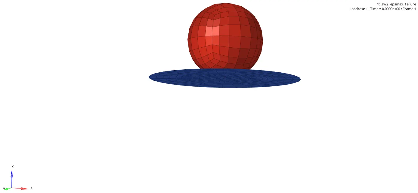
STEP 6: Checking the number of cycles it takes, energy error, mass error and simulation time.

• Number of cycles = 49380
• Energy error = 0.8%
• Mass error = 0.0
• Simulation time = Starter+Engine run time = 100.52 s

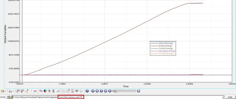
STEP 7: Switch to Hypergraph 2D, upload law2_epsmax_failure.T01

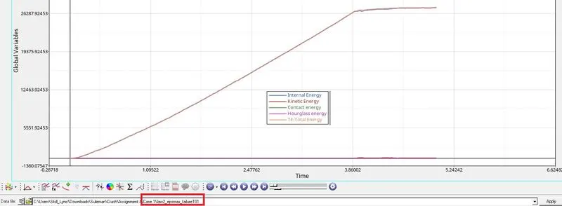
PROCEDURE FOR OBJECTIVE 2 :In Fail/Johnson collector changing ifail_sh=1, dadv=1, Ixfem=1 and running the model name as law2_epsmax_crack, observing simulation, discussing number of cycles it takes, energy error and plotting energies graph.

STEP 1: Import Case 1 Solver desk law2_epsmax_failure_0000.rad file

STEP 2: Change Failure_Johnson collector as per given challenge.

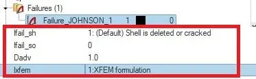
• Analysis>Radioss>save as input law2_epsmax_failure_0000.rad file
• Save path as --case2/law2_epsmax_crack0000.rad
• Checkbox include collectors
• Write (-nt 4) in options
• Click Radioss

STEP 3: Switch to Hyper view

STEP 4: select local model and result law2_epsmax_crack.h3d file

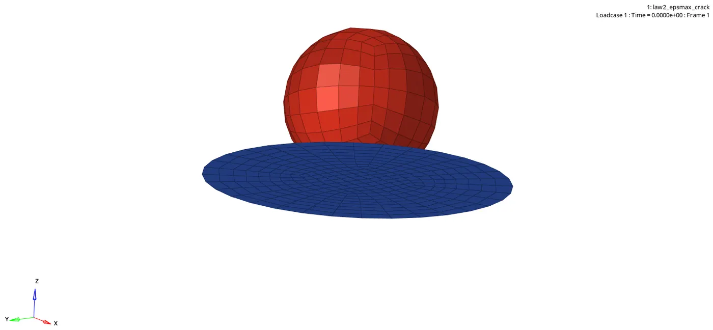
STEP 5: Checking the number of cycles it takes, energy error, mass error and simulation time.

• Number of cycles = 49217
• Energy error = 4.1%
• Mass error = 0.0
• Simulation time = Starter+Engine run time = 102.34s

STEP 6: Switch to Hypergraph 2D, upload law2_epsmax_crackT01 file

PROCEDURE FOR OBJECTIVE 3 : Deleting Fail/Johnson card, running the model name as law2_epsmax_nofail , observing simulation, discussing the number of cycles it takes, energy error, mass error and plotting energies graph.

STEP 1: Import Case 2 Solver desk law2_epsmax_crack_0000.rad file

STEP 2: Delete Failure_Johnson collector as per given challenge.

STEP 3:

• Analysis>Radioss>save as input law2_epsmax_nofail.rad file
• Save path as --case3/law2_epsmax_crack0000.rad
• Checkbox include collectors
• Write (-nt 4) in options
• Click Radioss

STEP 5: Switch to Hyper view

STEP 6: select local model and result law2_epsmax_nofail.h3d file

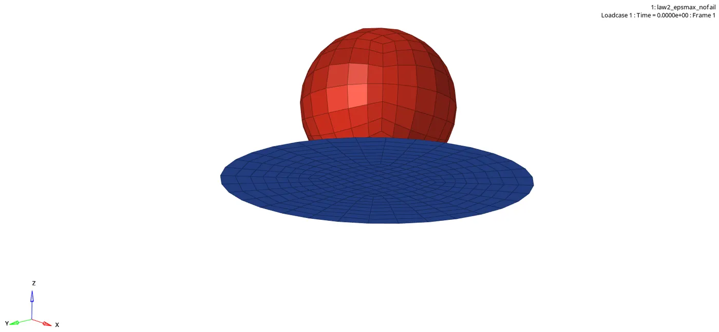
STEP 7: Checking the number of cycles it takes, energy error, mass error and simulation time.

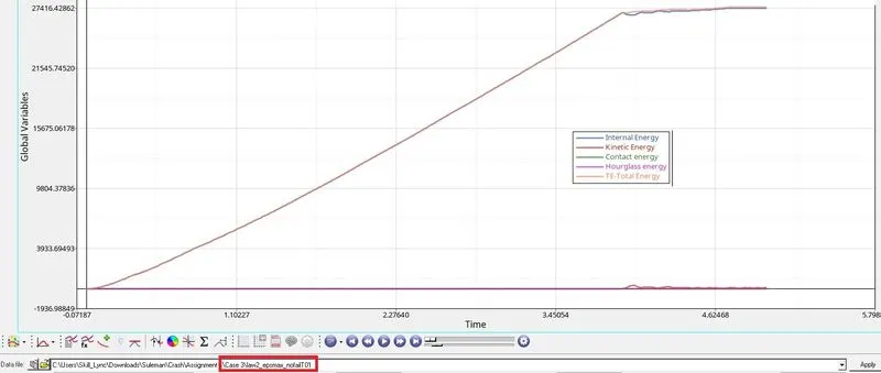
• Number of cycles = 49408
• Energy error = 0.8 %
• Mass error = 0.0
• Simulation time = Starter+Engine run time = 101.84s

STEP 8: Switch to Hypergraph 2D, upload law2_epsmax_nofailT01 file

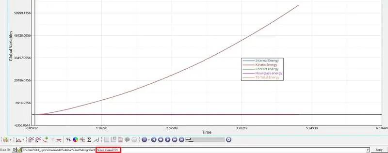
PROCEDURE FOR OBJECTIVE 4 : Deleting the value of esp_p_max_, running the model name as law2, observing simulation, discussing the number of cycles it takes, energy error, mass error and plotting energies graph.

STEP 1: Import Case 3 Solver desk law2_epsmax_nofail_0000.rad file

STEP 2: Delete value of esp_p_max_ from material collector as per given challenge.

STEP 3:

• Analysis>Radioss>save as input law2_epsmax_nofail.rad file
• Save path as --case4/law2_0000.rad
• Checkbox include collectors
• Write (-nt 4) in options
• Click Radioss

STEP 5: Switch to Hyper view

STEP 6: select local model and result law2l.h3d file

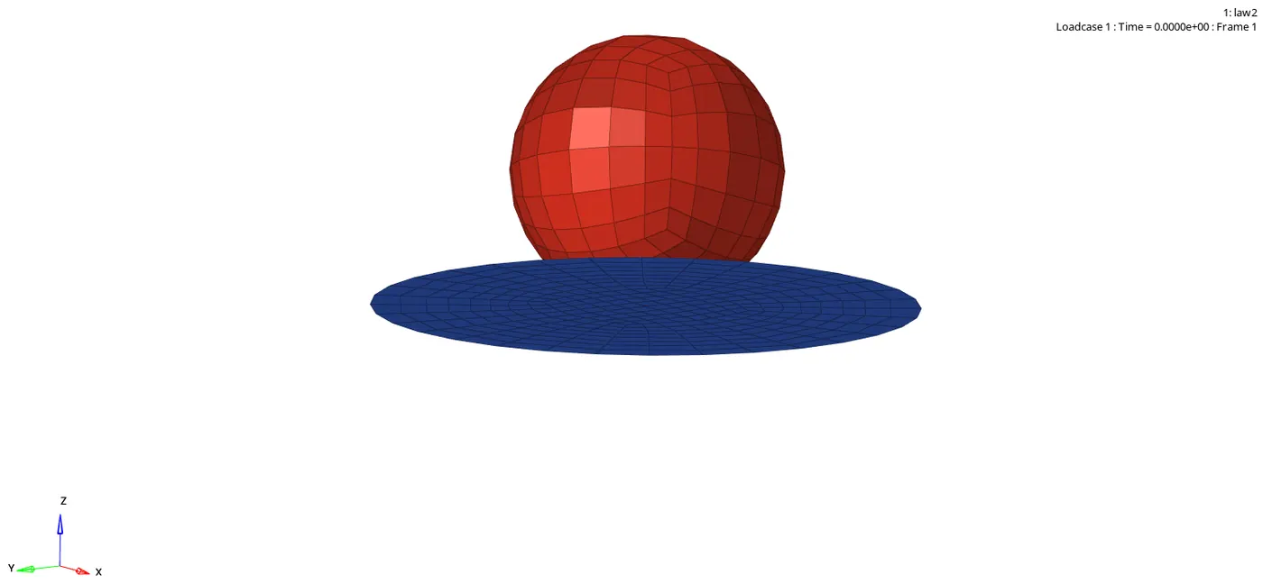
STEP 7: Checking the number of cycles it takes, energy error, mass error and simulation time.

• Number of cycles = 48737
• Energy error = 3.0 %
• Mass error = 0.0
• Simulation time = Starter+Engine run time = 99.95s

STEP 8: Switch to Hypergraph 2D, upload law2T01 file

PROCEDURE FOR OBJECTIVE 5 : Converting the material model to law1 elastic with same density, E, Nu, observing simulation, checking the number of cycles it takes, energy error, mass error and plotting energies graph.

STEP 1: Import Case 4 Solver desk law20000.rad file

STEP 2: converting the material model to lawas per given challenge.

STEP 3:

• Analysis>Radioss>save as input law1_0000.rad file
• Save path as --case5/law1_0000.rad
• Checkbox include collectors
• Write (-nt 4) in options
• Click Radioss

STEP 5: Switch to Hyper view

STEP 6: select local model and result law1.h3d file

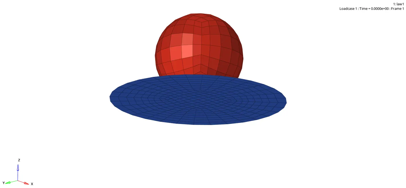
STEP 7: Checking the number of cycles it takes, energy error, mass error and simulation time.

• Number of cycles = 48851
• Energy error = - 9.6 % (negative)
• Mass error = 0.0
• Simulation time = Starter+Engine run time = 100.79s

STEP 8: Switch to Hypergraph 2D, upload law1T01 file

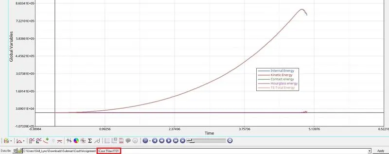
PROCEDURE FOR OBJECTIVE 6 : Converting the card to law36 elasto plastic based giving data as per given in challenge, observing simulation, checking the number of cycles it takes, energy error, mass error and plotting energies graph.

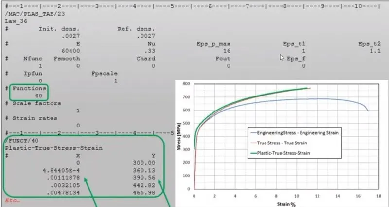
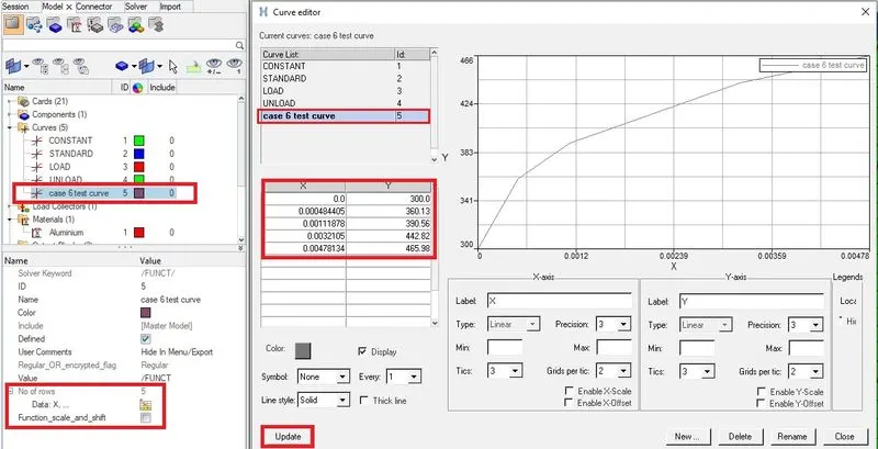
(Fig.1)

STEP 1: Import Case 5 Solver desk law1_0000.rad file

STEP 2: converting the material model to law36 and edit the parameters as per given challenge. (Fig.1)

STEP 3: Create a new curve in curves collector and rename it.

STEP 4: Give the X and Y coordinate as per given challenge. (Fig.1)

STEP 3:

• Analysis>Radioss>save as input law36_0000.rad file
• Save path as --case6/law36_0000.rad
• Checkbox include collectors
• Write (-nt 4) in options
• Click Radioss

STEP 5: Switch to Hyper view

STEP 6: select local model and result law36.h3d file

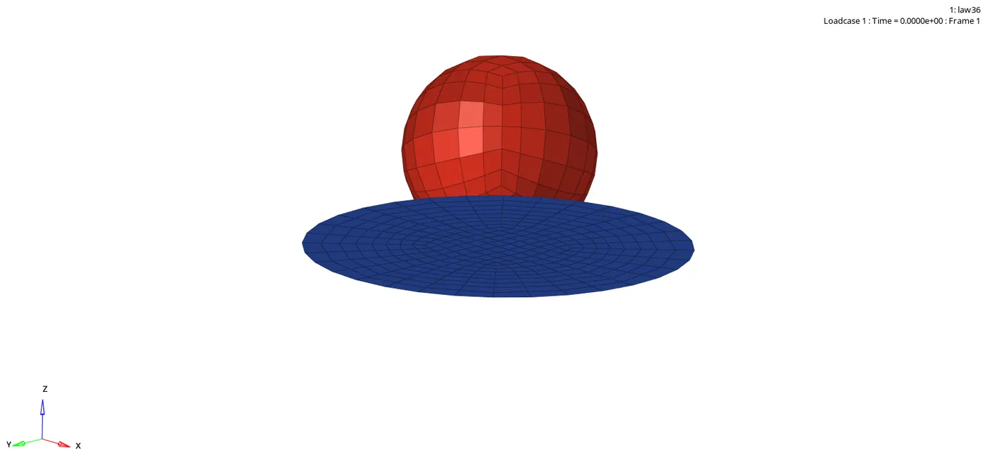
STEP 7: Checking the number of cycles it takes, energy error, mass error and simulation time.

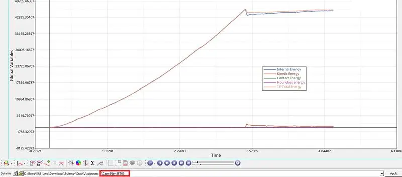
• Number of cycles = 53164
• Energy error = - 2.3 % (negative)
• Mass error = 0.0
• Simulation time = Starter+Engine run time = 111.51s

STEP 8: Switch to Hypergraph 2D, upload law36T01 file

PROCEDURE FOR OBJECTIVE 7 : Opening Law27_0000.rad, changing the shell properties to recommended shell property, running that model with law27 material card, observing simulation, checking the number of cycles it takes, energy error, mass error and plotting energies graph

STEP 1: Import Case 6 Solver desk law36_0000.rad file

STEP 2: Changing the shell properties on our own which can results best

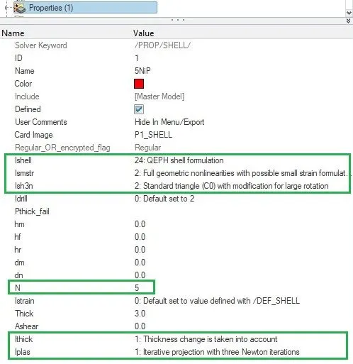
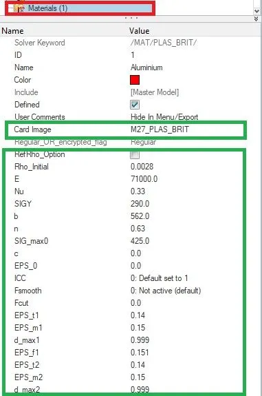
STEP 3: Convert the material model to law27 (M27_Plast_Brit) and edit the parameters which can results best in our own.

STEP 4:

• Analysis>Radioss>save as input law27_0000.rad file
• Save path as --case7/law27_0000.rad
• Checkbox include collectors
• Write (-nt 4) in options
• Click Radioss

STEP 5: Switch to Hyper view

STEP 6: select local model and result law27.h3d file

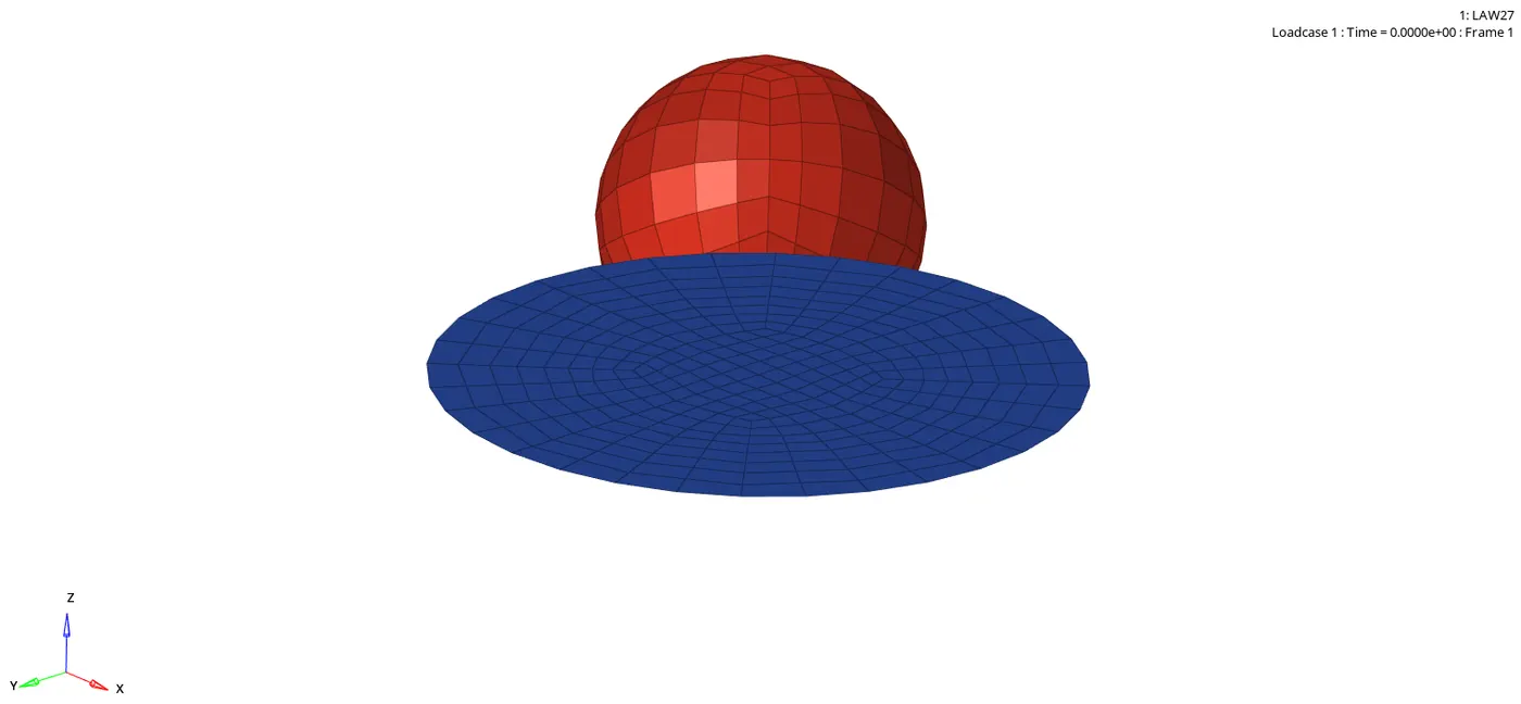
STEP 7: Checking the number of cycles it takes, energy error, mass error and simulation time.

• Number of cycles = 49501
• Energy error = 0.8 %
• Mass error = 0.0
• Simulation time = Starter+Engine run time = 106.95 s

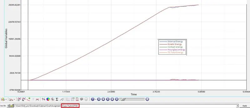
STEP 8: Switch to Hypergraph 2D, upload law27T01 file

RESULTS:

	No. of Cycles	Energy Error	Mass Error	Simulation Time
Case 1	49380	0.8 %	0.0	100.52 s
	Internal energy and total energy follows the same curve Kinetic energy and contact energy follows the same curve and were constant
Case 2	49217	4.1 %	0.0	102.34 s
	Internal energy and total energy follows the same curve Kinetic energy and contact energy follows the same curve and were constant
Case 3	49408	0.8 %	0.0	101.84 s
	Internal energy and total energy follows the same curve Kinetic energy and contact energy follows the same curve and were constant
Case 4	48737	3.0 %	0.0	99.95 s
	Internal energy and total energy follows the same curve linearly Kinetic energy and contact energy follows the same curve and were constant without any deviation
Case 5	48851	- 9.6 %	0.0	100.79 s
	Internal energy and total energy follows the same curve and then drops Kinetic energy and contact energy follows the same curve and were constant with small davition in end in KE
Case 6	53164	-2.3 %	0.0	111.51 s
	Internal energy and total energy follows the same curve linearly then drops and again follows Kinetic energy and contact energy follows the same curve and were constant with little deflection in KE
Case 7	49501	0.8 %	0.0	106.95 s
	Internal energy and total energy follows the same curve Kinetic energy and contact energy follows the same curve and were constant

COMPARISONS:

Case 1-2 : Case 1 is run as it is and case 2 we made changes in failure collector ifail_sh=1, dadv=1, Ixfem=1.

Number of cycles taken in case 1 is more as compared to case 2, we can see a huge energy error difference between them and time taken in case 1 is less than case 2.

Case 2-3: We Deleted Fail/Johnson card in case 3.

Number of cycles taken in case 3 is more as compared to case 2, here also we can see that the huge difference between energy error and time taken in case 3 is less than case 2.

Case 3-4: Deleting the value of esp_p_max_ in material card in case 4. Esp_p_max - Plastic strain beyond this will cause element deletion

Number of cycles taken in case 3 is more than case 3, energy error is 0.8 % and 3.0 % respectively, time taken in case 4 is less than case 3.

Case 4-5: Changing material model to law1 (M1_ELAST) in case 5, Law 1 elastic (Isotropic elasticity) - Isotropic means that a material have the same material properties in all 3 direction.

Number of cycles taken in case 5 is little more than case 4, energy error is negative and positive respectively and time taken in cse 4 is less than case 5.

Case 5-6: Changing material model to law36 (M36_PLAST_TAB) in case 6, Law 36 material law helps in modeling isotropic elasto plastic material using user defined function for the work hardening portion of the stress strain curve for different strain rates.

Number of cycles taken in case 5 is more than case 6, energy error is negative in both the cases and simulation time is taken less in case 5.

Case 6-7: Changing material model to law27 (M27_PLAST_BRIT) in case 7, Law 27 has isotropic elasto-plastic material law with orthotropic brittle failure model. Orthotropic materials differ along three manually orthogonal axes. Here material damage and failure happens only in tensions.

Number of cycles taken in case 6 is more than case 7, energy error is negative and positive respectively and simulation time taken in case 6 is more than case 7.

LEARNINGS:

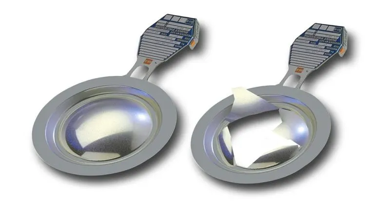
• Rupture Plate

A rupture disc is a non-closing pressure relief, pressure safety disc, burst disc, bursting disc, or burst diaphragm device used to protect industrial applications from overpressure- or vacuum-related events. It is a non-closing pressure relief device used to protect industrial applications from overpressure- or vacuum-related events.

• Importing starter file runname_0000.rad file
• Using Radioss command
• Running runnane.h3D file in Hyperview to see animation
• Reading runname_0001.out file
• Using Hypergraph 2D
• Writing curves coordinate in a curves collector.
• Observing Energies graph
• Changing properties and material parameters
• Details on Material Card Image law1(m1_elast), law36(m36_plast_tab), law27(m27_plast_brit).