Analysis of the crash simulations of Rupture Plate model using RADIOSS solver in HyperWorks according to 7 different material settings.

PROJECT REPORT

SKILL LYNC ASSIGNMENT 4

Aim:

To run the crash simulations of the given model using RADIOSS solver in HyperWorks according to 7 different settings of materials etc, and compare the results using values obtained from the solver and graphical plots of different kinds.

Objective:

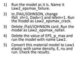
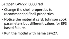
Various properties are to be changed as per the following :

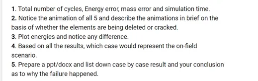
The results of the above results are to be compared on the basis of:

Theory:

What is RADIOSS?

Altair RADIOSS is a multidisciplinary finite element solver developed by Altair Engineering.^[1] It can solve both linear and non-linear problems. It is a finite element solver using implicit and explicit integration schemes for the solution of engineering problems, from linear statics and linear dynamics to nonlinear transient dynamics and mechanical systems. This multidisciplinary solver enables designers to maximize performance related to durability, NVH, crash, safety, manufacturability, and fluid-structure interaction, in order to bring products to market faster.

RADIOSS’ analysis capabilities for linear and non-linear finite element analysis, sheet metal stamping, and multi-body dynamics are accessible via two input formats.

What is Finite Element Analysis?

Finite element analysis (FEA) is the process of simulating the behaviour of a part or assembly under given conditions so that it can be assessed using the finite element method (FEM). FEA is used by engineers to help simulate physical phenomena and thereby reduce the need for physical prototypes, while allowing for the optimisation of components as part of the design process of a project.

FEA uses mathematical models to understand and quantify the effects of real-world conditions on a part or assembly. These simulations, which are conducted via specialised software, allow engineers to locate potential problems in a design, including areas of tension and weak spots.

What is a time step in FEA?

In the context of explicit analysis, time step is the time required for a shock wave to propagate across the smallest distance of the element. A run is a single model simulation and it starts at time zero and continues till the user defined endpoint is reached. The basic time unit in the run is the time step.The time step is directly dependent on the length of the element and inversely proportional to the speed of sound of material. The speed of sound of the material is dependent on both material modulus and density of the material. So, if the material is stiffer (higher modulus of elasticity), the speed of sound increases resulting in a lower solution time step.

Materials in HyperWorks

Choosing the right material and providing the reliable material data in performing a simulation is very important. RADIOSS provides one of the most comprehensive material and rupture libraries in the industry. The material laws and rupture criteria span across definitions for concrete, foam, rubber, steel, composites, biomaterials, and more. The choice of a constitutive law for a given material depends at first to desired quality of the model.

The available material laws classification is as follows:

• Isotropic Elastic
• Isotropic Elasto-Plastic
• Composite and Fabric
• Hyper and Visco-elastic
• Concrete and Rock
• Honeycomb
• Hydrodynamic
• Multi-Material, Fluid and Explosive

In this project we will have a look at the following material laws:

• Law 1 – Elastic
• Law 2 – Johnson-Cook
• Law 25 – Composite
• Law 27 – Elastic-Plastic Brittle
• Law 28 – Honeycomb
• Law 36 – Elastic-Plastic Tabulated
• Law 42 – Ogden (Hyperelastic)
• Law 69 – Ogden & Mooney-Rivlin (Hyperelastic)
• Law 70 – Foam

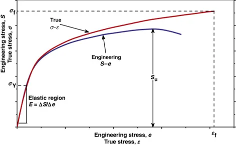
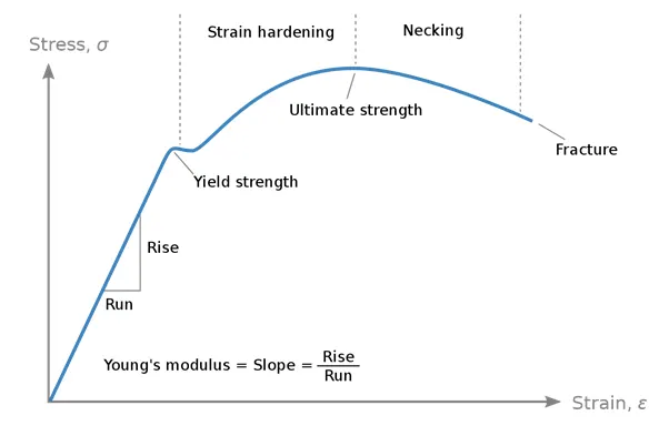
The stress-strain curve:

Some of the important terms and definitions pertaining of the stress-strain analysis is given below:

Elastic Range: The limit of strain produced on the material up to which original shape of the material can be restored is considered as elastic range. On application of force in elastic range material restores its shape once the force is removed.

Proportional Limit: Its a point on the stress-strain curve up to which stress in proportional to strain.

Stress strain curve yield point is the material property defined as the stress at which a material begins to deform plastically. Prior to the yield point the material will deform elastically and will return to its original shape when the applied stress is removed. Once the yield point is passed, some fraction of the deformation will be permanent and non-reversible.

The yield point determines the limits of performance for mechanical components, since it represents the upper limit to forces that can be applied without permanent deformation.

The mechanical strength of the material corresponding to yield point is defined as yield strength.

When the stress is sufficient to permanently deform the metal, it is called plastic deformation. The plastic region is the portion where some permanent deformation will occur, even if the load is removed.

Failure point is when the specimen fractures.

Ductile materials, which includes structural steel and many alloys of other metals, are characterized by their ability to yield at normal temperatures.

Brittle materials, which includes cast iron, glass, and stone, are characterized by the fact that rupture occurs without any noticeable prior change in the rate of elongation.

When the load on a wire is increased beyond the yield point, the stress developed exceeds the yield strength. If the load is removed after this point, the body does not regain its origin volume but gets a little deformed. Here, strain is non-zero even if the stress is zero. This property of the material is known as the permanent set and the deformation is called plastic deformation.

Yield strength refers to an indication of maximum stress that can be developed in a material without causing plastic deformation. It is the stress at which a material exhibits a specified permanent deformation and is a practical approximation of the elastic limit

Given below are the basic Engineering stress vs True stress diagram and , the basic Stress-Strain diagram:

Material Laws:

1. /MAT/LAW1 (ELAST)

Linear Elastic Material /MAT/ELAST defines an isotropic, linear elastic material using Hooke’s law. This law represents a linear relationship between stress and strain. It is available for truss, beam (type 3 only), shell and solid elements. This material law is used to model purely elastic materials. The material stiffness is determined by only two values: the Young’s modulus (E), and Poisson’s ratio (n).

2. /MAT/LAW2 (PLAS_JOHNS)

Johnson-Cook Material This law represents an isotropic elasto-plastic material using the Johnson-Cook material model. This model expresses material stress as a function of strain, strain rate and temperature. A built-in failure criterion based on the maximum plastic strain is available.

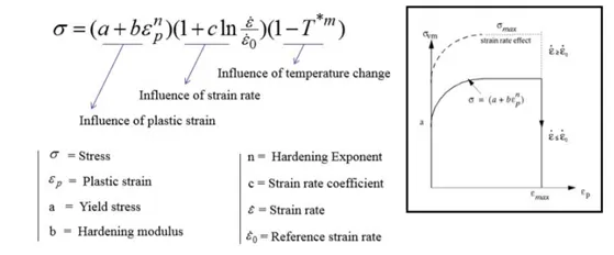
3. /MAT/LAW2 or /MAT/JOHNS: [Optional Failure Model]

Using the Johnson-Cook failure model /FAIL/JOHNSON along with the Johnson-Cook material model provides more user control of the failure Johnson-Cook failure strain definition:

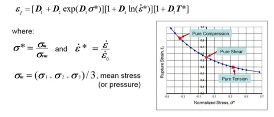
4. /MAT/LAW36 (PLAS_TAB) [Elastic Plastic Piecewise Linear Material]

This law models an isotropic elasto-plastic material using user-defined functions for the workhardening portion of the stress-strain curve (for example, plastic strain vs. stress) for different strain rates. Note: The first point of yield stress functions (plastic strain vs stress) should have a plastic strain value of zero. If the last point of the first (static) function equals 0 in stress, default value of ep-max is set to the corresponding value of ep.

5. /MAT/LAW27 (PLAS_BRIT) [Elasto-Plastic Material with Brittle Failure]

This law combines an isotropic elasto-plastic Johnson-Cook material model with an orthotropic brittle failure model. Material damage is accounted for prior to failure. Failure and damage occur only in tension. This law is applicable only for shells.Yield surface definition same as Johnson-Cook (Law2) Useful for modeling brittle failure of glass.

6. /MAT/OGDEN or /MAT/LAW42 [Ogden, Mooney-Rivlin]

Visco Hyperelastic behavior (non-linear elastic) is generally used to model incompressible rubbers, polymers, foams, and elastomers. This material can be used with shell and solid elements

7. /MAT/LAW69 [Incompressible Hyperelastic]

Material model specified using the Ogden or MooneyRivlin material models. It is generally used to model incompressible rubbers, polymers, foams, and elastomers. Material parameters are computed from engineering stress-strain curve from uniaxial tension and compression tests. It is used with shell and solid elements. Users can reproduce viscous behavior in this material card using /VISC/PRONY card, which is an isotropic visco-elastic Maxwell model that can be used to add visco-elasticity to certain shell and solid element material models. The visco-elasticity is input using a Prony series

Failure Models

In addition to the possibility to define user's material failure models, Radioss integrates several failure models. These models use generally a global notion of cumulative damage to compute failure. They are mostly independent to constitutive law and the hardening model and can be linked to several available material laws

Given Model:

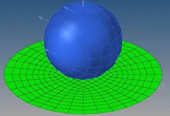
The given model here is a ball which would be crashing into a circular plate during the simulations.

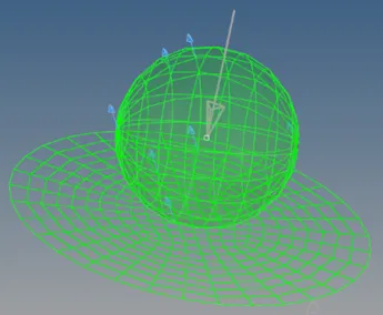
Case 1:

Steps:

1. Export the model and save the model file with the name Law1_epsmax_failure.
2. Run the model on the Radioss solver as it is without making any changes in the properties.
3. Plot the Von Mises Contour and different Energy plot.

Given Below is the Materials Card of the given case:

The unit system in all the values written below is [kg mm ms]

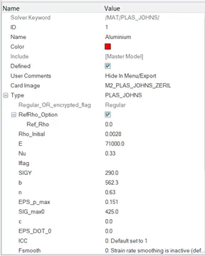
On running the Radioss solver .out file was created in the directory from where different values were noted down:

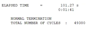
Elapsed time: 101.27 seconds

Total No of Cycles: 49380

Energy error: 0.8%

Mass Error: 0.000

The energy error and the mass error look well within the limits.

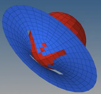
On running the animation of HyperWorks, we get the following way of crashing on different points of times:

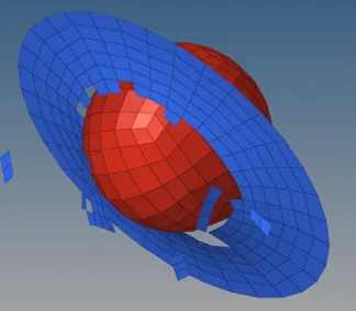
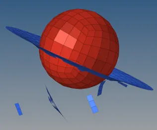
The contour plot of the Von Mises stress is given below:

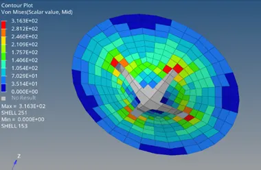
Here we can notice the stresses on different elements in different colours during the animation. The stress distribution here is dependent on the values of Material cars and shell element properties defined above.

Maximum Von Mises Stress: 3.163E+02

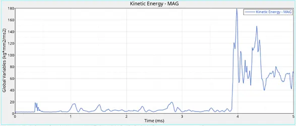
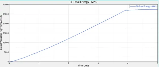
Different Energy Plots are given below, these were not plotted on a single graph because the value of changes in the Kinetic Energy is quite small and hence was not noticeable on the same graph as that of Internal Energy:

Internal Energy: 0.2730E+05

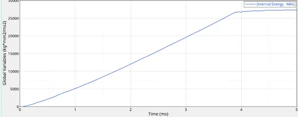
Kinetic Energy: 67.81 (Final Value)

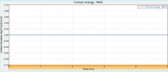
Contact Energy:

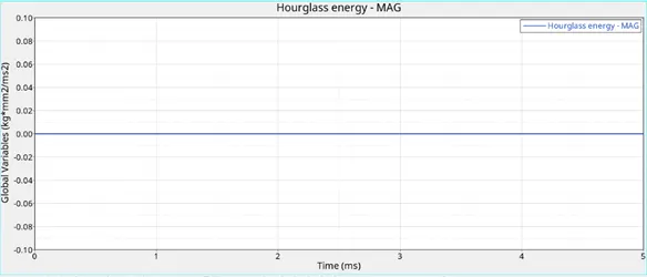
Hourglass Energy:

Total Energy:

Case 2:

Steps:

1. Export the model and save the model file with the name Law1_epsmax_crack
2. Change the values of parameters (given below) as asked in the objective.
3. Run the model on the Radioss solver.
4. Plot the Von Mises Contour and different Energy plots

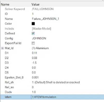
Given Below is the Faliure Card of the given case:

The unit system in all the values written below is [kg mm ms]

Here, in this card the following values were changed in /FAIL/JOHNSON:

For crack formulation: Ixfem=1

Crack Advancement Criterion : Dadv=1

Shear failure flag : Ifail_sh=1

On running the Radioss solver .out file was created in the directory from where different values were noted down:

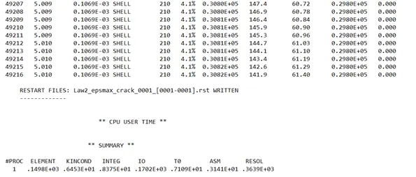
The Radioss solver is as follows:

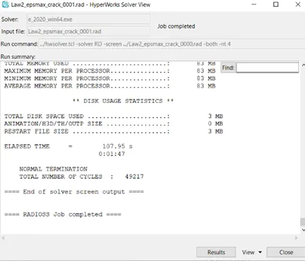
Elapsed time: 107.95 seconds

Total No of Cycles: 49217

Energy error: 4.1%

Mass Error: 0.000

The mass error is 0 and perfect but the energy error is 4.1% which is quite higher value and is going out of the limits.

On running the animation of HyperWorks, we get the following way of crashing:

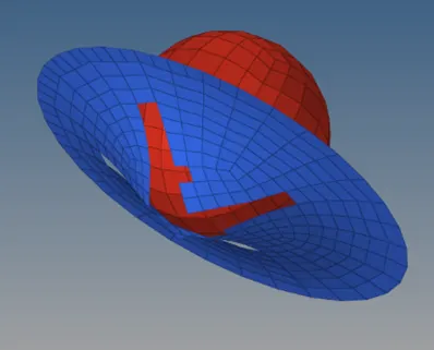
The contour plot of the Von Mises stress is given below:

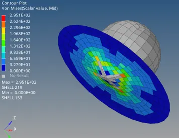
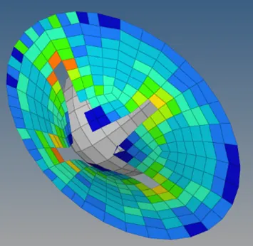
Here we can notice the stresses on different elements in different colours during the animation. The stress distribution here is dependent on the values of Material cars and shell element properties defined above.

Maximum Von Mises Stress: 2.951E+02

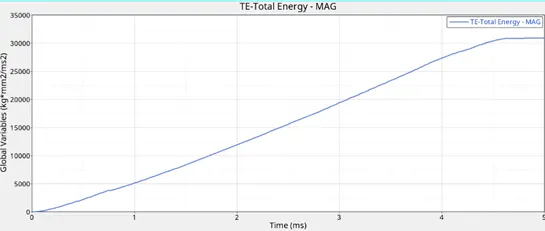
Different Energy Plots are given below, these were not plotted on a single graph because the value of changes in the Kinetic Energy is quite small at some points and hence was not noticeable on the same graph as that of Internal Energy:

Internal Energy: 0.3082E+05

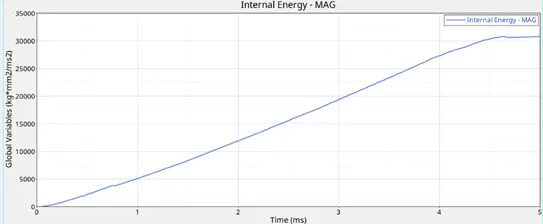
Kinetic Energy:141.9 (Final Value)

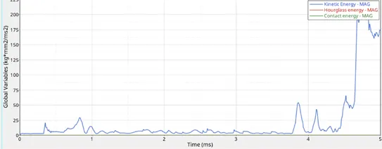
Total Energy:

Case 3:

Steps:

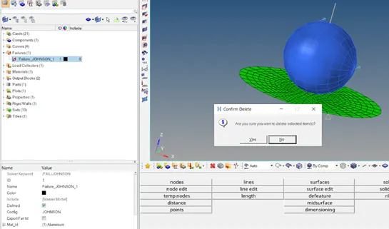
1. Export the model and save the model file with the name Law1_epsmax_fail.
2. Delete the /FAIL/JOHNSON card.
3. Run the model on the Radioss solver.
4. Plot the Von Mises Contour and different Energy plots.

The unit system used in all the values written below is [kg mm ms]

On running the Radioss solver .out file was created in the directory from where different values were noted down:

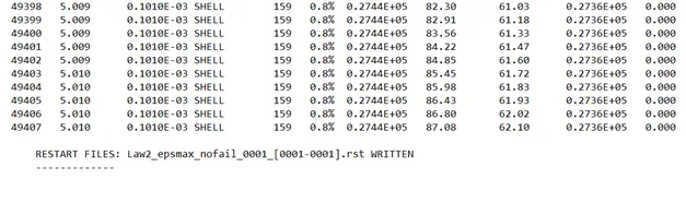
The Radioss solver is as follows:

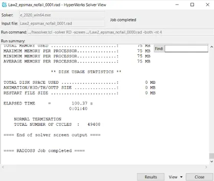
Elapsed time: 100.37 seconds

Total No of Cycles: 49408

Energy error: 0.8%

Mass Error: 0.000

The Energy Error here looks very near to 0 and seems within the limits.

On running the animation of HyperWorks, we get the following way of crashing:

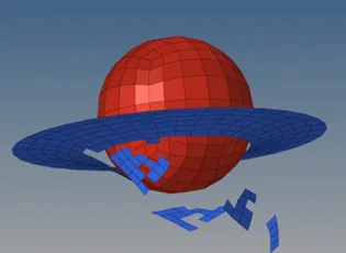
Von Mises Contour:

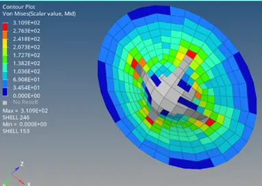
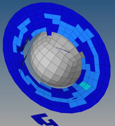
Here we can notice the stresses on different elements in different colours during the animation. The stress distribution here is dependent on the values of Material cars and shell element properties defined above.

Maximum Von Mises Stress: 3.163E+02

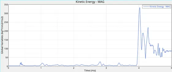
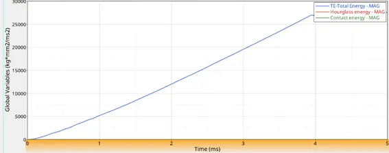
Different Energy Plots are given below, these were not plotted on a single graph because the value of changes in the Kinetic Energy is quite small and hence was not noticeable on the same graph as that of Internal Energy:

Internal Energy: 0.2744E+05

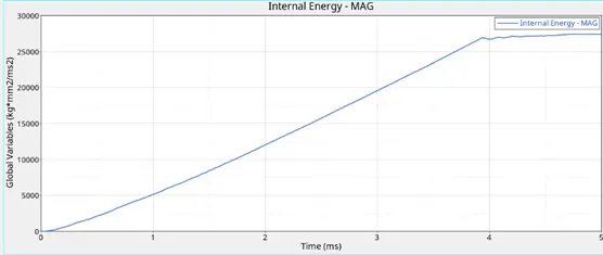
Kinetic Energy: 87.08 (Final Value)

Total Energy:

Case 4:

Steps:

1. Export the model and save the model file with the name Law2.
2. Delete the /FAIL/JOHNSON failure card as before.
3. Set the value of Eps_max as 0
4. Run the model on the Radioss solver.
5. Plot the Von Mises Contour and different Energy plots.

On running the Radioss solver .out file was created in the directory from where different values were noted down:

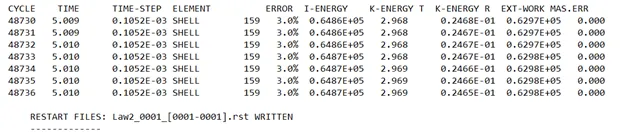
The RADIOSS solver is as follows:

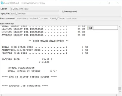
Elapsed time: 96.45 seconds

Total No of Cycles: 48737

Energy error: 3.0%

Mass Error: 0.000

Mass error is 0 which is perfect, but energy error is though almost very less i.e. 3% but still is not much acceptable.

On running the animation of HyperWorks, we get the following way of crashing:

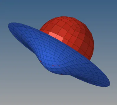
The contour plot of the Von Mises stress is given below:

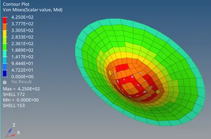
Here we can notice the stresses on different elements in different colours during the animation. The stress distribution here is dependent on the values of Material cars and shell element properties defined above.

Maximum Von Mises Stress: 4.25 E+02

Different Energy Plots are given below, these were not plotted on a single graph because the value of changes in the Kinetic Energy is quite small and hence was not noticeable on the same graph as that of Internal Energy:

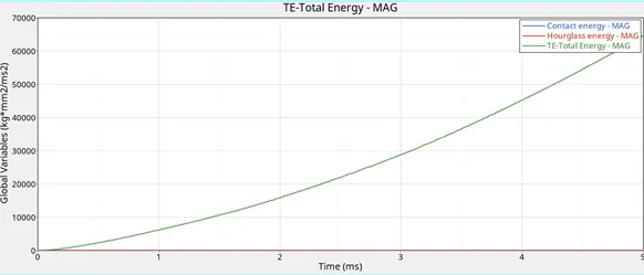
Internal Energy: 0.6487E+05

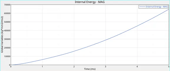
Kinetic Energy: 2.969

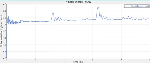
Total Energy:

Case 5:

Steps:

1. Export the model and save the model file with the name Law1
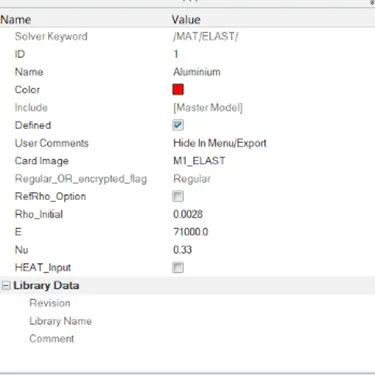
2. Change the material to M1_ELAST keeping all other property values same
3. Run the model on the Radioss solver.
4. Plot the Von Mises Contour and different Energy plots.

The material card is given below and it can be noticed that the Card Image was changed:

On running the Radioss solver .out file was created in the directory from where different values were noted down:

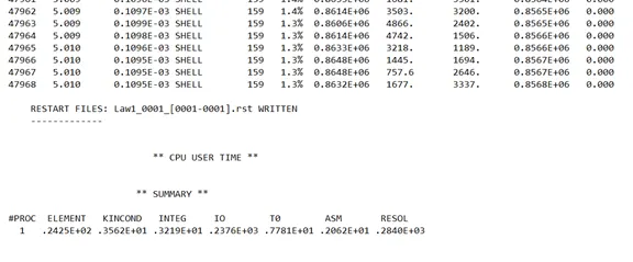
The RADIOSS solver is as follows:

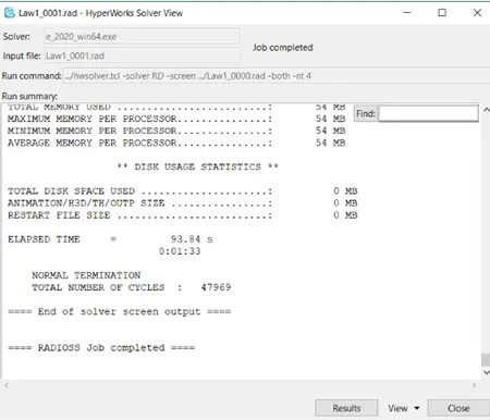
Elapsed time: 93.84 seconds

Total No of Cycles: 47969

Energy error: 1.3%

Mass Error: 0.000

Mass Error and energy error seem well within the limits,

On running the animation of HyperWorks, we get the following way of crashing on different points of times:

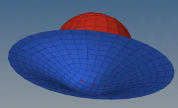
Von Mises Contour Plot:

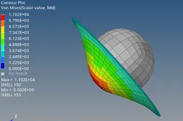
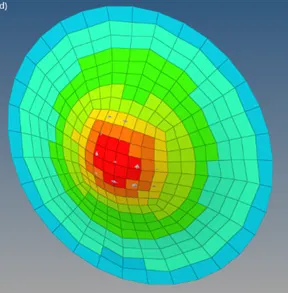
Here we can notice the stresses on different elements in different colours during the animation. The stress distribution here is dependent on the values of Material cars and shell element properties defined above.

Maximum Von Mises Stress: 1.102E+04

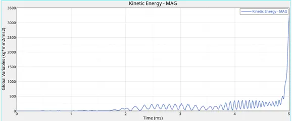
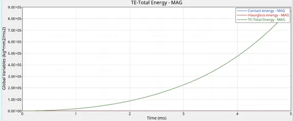
Different Energy Plots are given below, these were not plotted on a single graph because the value of changes in the Kinetic Energy is quite small and hence was not noticeable on the same graph as that of Internal Energy:

Internal Energy: 0.8632E+06

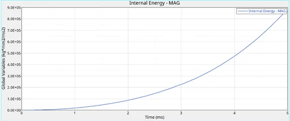
Kinetic Energy: 1677

Total Energy:

Case 6:

Steps:

1. Export the model and save the model file with the name Law27.
2. The properties here were changed to the recommended properties.
3. Run the model on the Radioss solver.
4. Plot the Von Mises Contour and different Energy plots.

The values in the material card given below were kept as it is:

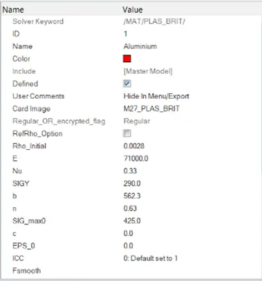
The values in the property card below were changed to recommended shell properties:

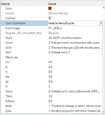
On running the Radioss solver .out file was created in the directory from where different values were noted down:

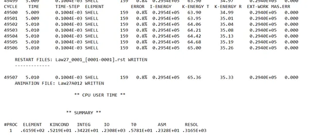
The RADIOSS solver is as follows:

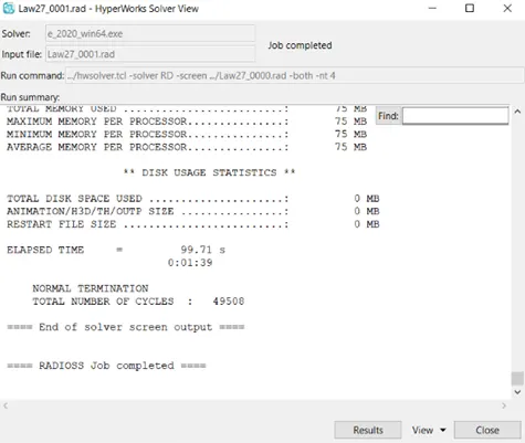
Elapsed time: 99.71 seconds

Total No of Cycles: 49508

Energy error: 0.8%

Mass Error: 0.000

Both energy error and mass error are well within the limits.

On running the animation of HyperWorks, we get the following way of crashing:

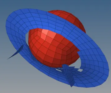
Von Mises Contour Plot:

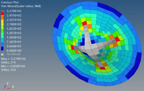
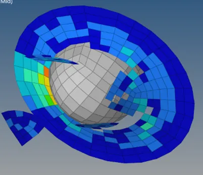
Here we can notice the stresses on different elements in different colours during the animation. The stress distribution here is dependent on the values of Material cars and shell element properties defined above.

Maximum Von Mises Stress: 3.279E+02

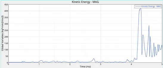
Different Energy Plots are given below, these were not plotted on a single graph because the value of changes in the Kinetic Energy is quite small and hence was not noticeable on the same graph as that of Internal Energy:

Internal Energy: 0.2954E+05

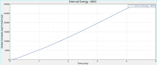
Kinetic Energy: 65 (Final Value)

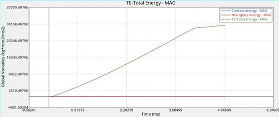
Total Energy:

Case 7:

Steps:

1. Export the model and save the model file with the name Law36
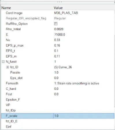
2. The card image in the Material is changed to M36_PLAS_TAB
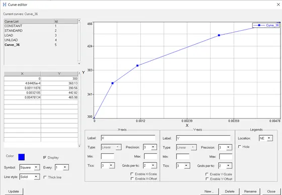
3. A new stress strain curve was created using the acutal values discussed.
4. Run the model on the Radioss solver.
5. Plot the Von Mises Contour and different Energy plots.

The material card is given below in which the card image is changed, the values of properties are entered and then the curve was assigned in fct_ID

The curve editor is as follows, the values of x and y are given accordingly:

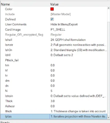
The property values were changed to recommended shell values as shown below:

On running the Radioss solver .out file was created in the directory from where different values were noted down:

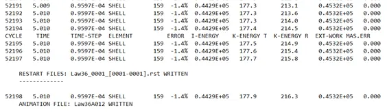
Radioss Solver is as follows:

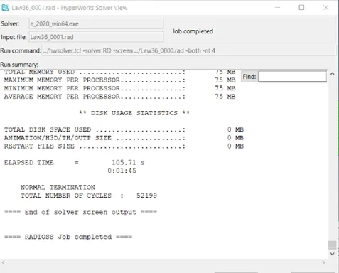
Elapsed time: 105.71 seconds

Total No of Cycles: 52199

Energy error: -1.4%

Mass Error: 0.000

This is the only case in this report where the nergy error is negative i.e the energy is getting decreased.

On running the animation of HyperWorks, we get the following way of crashing on different points of times:

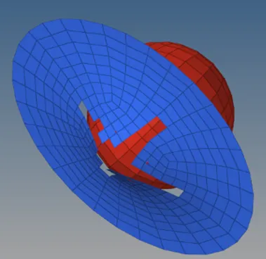
Von Mises Contour Plot:

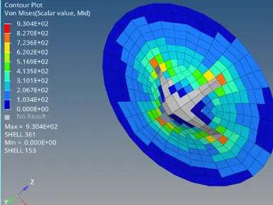
Here we can notice the stresses on different elements in different colours during the animation. The stress distribution here is dependent on the values of Material cars and shell element properties defined above.

Maximum Von Mises Stress: 9.304E+02

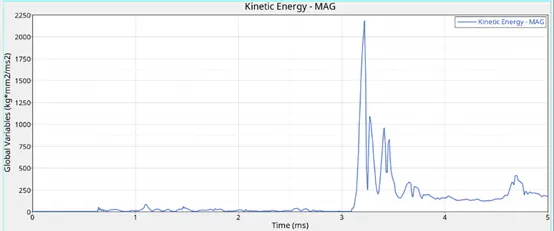
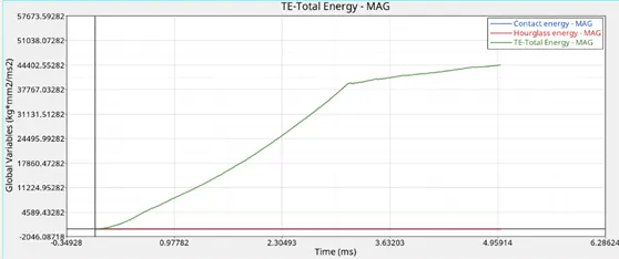
Different Energy Plots are given below, these were not plotted on a single graph because the value of changes in the Kinetic Energy is quite small and hence was not noticeable on the same graph as that of Internal Energy:

Internal Energy: 0.4429E+06

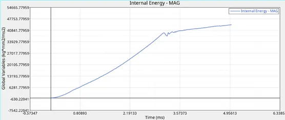
Kinetic Energy: 177.7 (Final Value)

Total Energy:

Results/Outcomes:

Case	Energy Error (%)	Mass Error (%)	Internal Energy (J)	Kinetic Energy (J)	Von Mises Stress (MPa)
1	0.8	0	0.2730E+05	67.81	316.3
2	4.1	0	0.3082E+05	141.9	295.1
3	0.8	0	0.2744E+5	87.08	310.9
4	3.0	0	0.6487E+5	2.969	425.0
5	1.3	0	0.8632E+6	1677	11020
6	0.8	0	0.2954E+6	65	327.9
7	-1.4	0	0.4429E+6	177.7	930.4

7 cases using Law1, Law2, Law 27 and Law 36 were tested at several values of different parameters and the results found were different from each other.

The Energy error was minimum in Cases 1, 3 and 6 i.e. 0.8%, so these cases are better than the others as far as energy fluctuation is concerned. Out of these also case 3 has the lowest value of Von Mises Stress on elements, so Case 3 can be a good option to use. Also, the overall Von Mises stress of Case 2 is lowest, so it is also a good case for application. Also, in case 2 Ixfem and Dadv values are 1 so a better crack propagation is obtained, there’s some plastic behaviour.

The Contact energy and Hourglass energy values were 0 in both the cases throughout.

Conclusions:

After running simulations for all 7 cases with appropriate values, different results were obtained. Contours and Energy graphs were plotted and the values were accordingly extracted and compared.