Aim: To run the simulation of ruptured plate using different material & property cards, analyzing & comparing the results obtained in different cases

Objectives of project:

1.To carry out ruptured plate simulation with various types of material and failure cards

2.To interpret and compare the stress contours and energy plots of the different cases

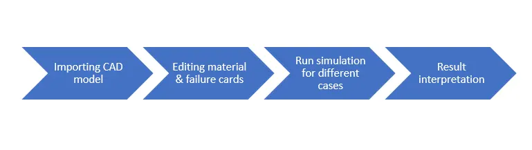
Workflow

Theoretical Aspects

Stress-Strain Curve

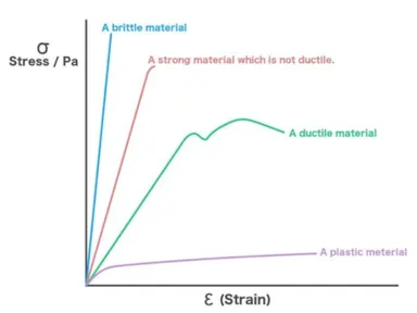
1. Brittle material: This material is considered strong because there is little strain for a high stress value, but this strength comes with the cost that it has no plastic region deformation. To be precise, the fracture of a brittle material is sudden with little or no deformation e.g. Glass
2. A strong material which is not ductile: steel wires stretch very little and break suddenly
3. Ductile material: After the elastic region there is a strange section where necking occurs i.e. permanent deformation occurs in this ‘plastic region’
4. A plastic material: Very small elastic region

Note:

1. A ductile material has a large elastic region
2. A plastic material has exceedingly small region in elasticity but a very large region in plasticity

If both materials are combined, you get a elastic-plastic material; the stress-strain curve for elastic-plastic material is as follows:

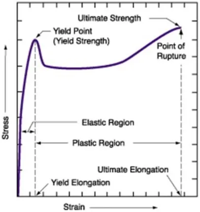
The strain at the point of rupture is the plastic strain at failure(eps_max). This is an important point because it is used in each and every material model wherever we want to see any kind of failure during crash analysis.

Isotropic Elasticity

1. Keyword /MAT/ELAST defines an isotropic linear elastic material using Hooke’s Law. This law represents linear relationship between stress & strain. It’s available for truss, beam(only type 3), shell and solid elements. Useful for elements attached to rigid body
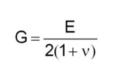
2. This material law is used to model purely elastic materials. To define this card we need only the values of: Young’s modulus, Poisson’s ratio, density. Modulus of rigidity can be computed using:

Note: Law 1 should not be used for parts undergoing large deformation. It’s important to avoid elastic materials while you are doing crash analysis. While, for a vibration or simple static structural analysis, you can go for elastic materials

In crash applications, the plastic region becomes very crucial and because it is made up of metallic materials or alloys usually even the elastic material is long enough. This creates a need to introduce a material: Isotropic Elasto-Plastic Materials

Isotropic Elasto-plastic Material

The most commonly used material laws are as follows:

Cowper-Symonds finds applicative wind shields

/MAT/LAW2(PLAS_JOHN) Johnson-Cook Material Model

1. This law represents an isotropic elasto-plastic material using the Jonson-Cook material model. This model expresses material stress as a function of strain, strain rate and temperature. A built-in failure criteria based on the maximum plastic strain is available(eps_max)

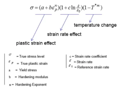
2. In case of crash, the temperature change is assumed to be negligible though in reality the temperature change is considerable, thus, the third term of temperature change evaluates to 1

3.If material is not temperature and strain rate sensitive, then both strain rate and temperature change terms evaluate to 1

Ixfem

This parameter represents the cracking of an element. Without using I_xfem treatment, the element will simply get deleted wherever you should have seen a crack. I_xfem gives room for even more realistic simulation.

The main challenge that is faced in using this treatment is that your material model must be very accurate. This is recommended for shorter propagations of crack i.e. it is not efficient to use when you want to see how a crack is propagating over a long distance.

Moreover, these can be used only for shell elements.

/MAT/LAW36(PLAS_TAB) Elasto-Plastic Piece-Wise Linear Material

1. In this law, we put in the lab recorded data of stress-strain curve which is generated from the material’s lab test. Being closer to lab obtained curve gives better simulation results

2. This is preferred over Johnson-Cook because in real life it is difficult to tell the failure criteria exactly thus, Johnson-Cook curve incorporates a lot of approximations which leads to deviation from lab data

3. Most used material model in industry

4. This law models an isotropic elasto-plastic material using user-defined functions for the work hardening portion of the stress-strain curve(plastic strain vs plastic stress) for different strain rates

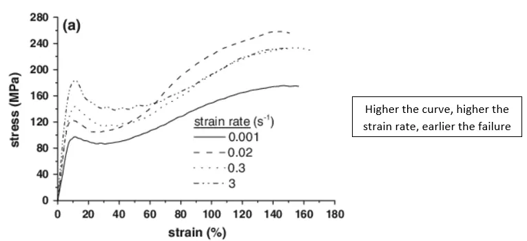
1. Available for brick and shell elements
2. Material plasticity curves can be given for an arbitrary no. of strain rates
3. It involves linear interpolation of stress-strain curve
4. To avoid poor curve extrapolation during strain calculation, a dummy curve can be defined for high strain rate value (can be put as the highest strain rate curve)
5. The curves must be defined such as they do not interest themselves in the strain range being used, otherwise the calculation may fail.

Damage and rupture parameters

1. is the maximum plastic strain for element deletion for any loading(tensile, compression or compression)
2. is the beginning of tensile damage. From this point the curve falls down to zero stress value but it reaches
3. is the end of tensile damage. The stress value is said is null but the element is not deleted
4. is the tensile failure strain value for element deletion

After deletion of the element, there is no coming back. So, the energy that gets absorbed in the elements gets dissipated or to be precise gets wasted i.e. it won’t remain in the solution anymore. That is why in the solver run you’ll see the energy fluctuation as and when the elements are getting deleted from the system.

/MAT/LAW36: Yield stress vs pressure

1. If the yield stress is pressure dependent, then a scale factor can be applied via a function, fct_ldp
2. Function fct_Idp is used to distinguish the behavior in tension & compression for certain materials(i.e. pressure dependent yield)
3. Function fct_Idp is used to distinguish the behavior in the tension and compression for certain materials(i.e. pressure dependent yield)

/MAT/LAW27(PLAS_BRIT) Elasto-Plastic Material with Brittle Fracture

This is a special material card for brittle materials

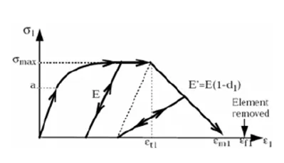
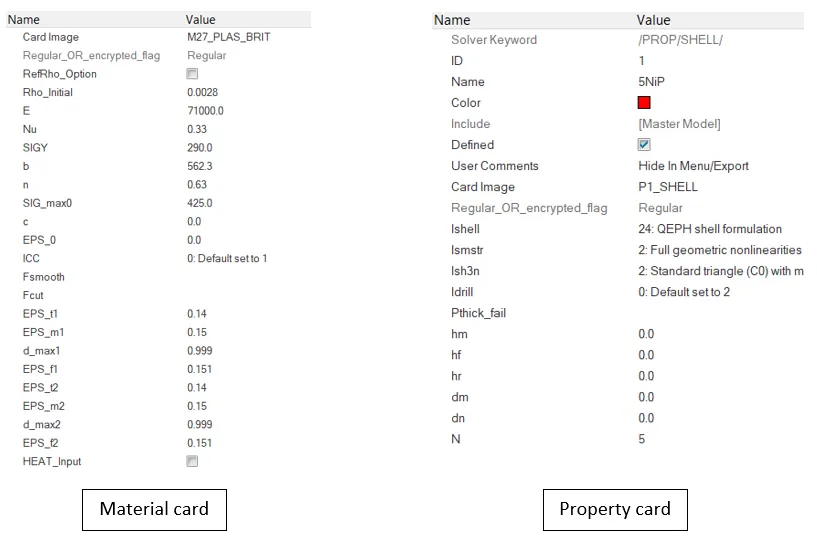
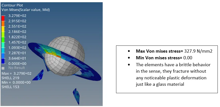
This law combines an isotropic elasto-plastic Jonson-Cook material model with orthotropic brittle failure model. Material damage is accounted for prior to failure. Failure and damage occur only in tension. This law is only applicable for shells

Yield surface definition same as Johnson-Cook(Law 2)

Damage and rupture defined with 4 parameters for each principal direction:

1. `ε_t`= strain at beginning of tensile failure
2. `ε_m`= Maximum tensile strain at which the stress value dropped to zero(as shown in above diagram)
3. D_max = Maximum damage factor
4. `ε_f`= Maximum tensile strain for element deletion

This law is useful for modelling brittle failure of glass

D_max is accelerating your element removal process. The path from the point to zero stress point will be accelerated

note: All the units are in: Kg mm ms

Model Provided

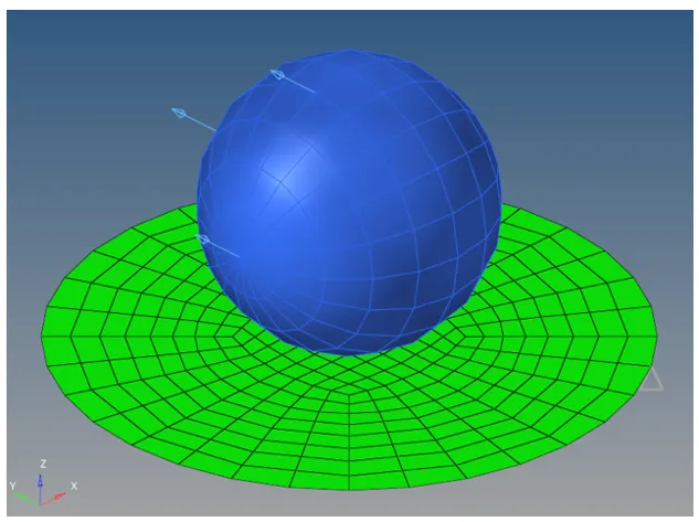
Case 1

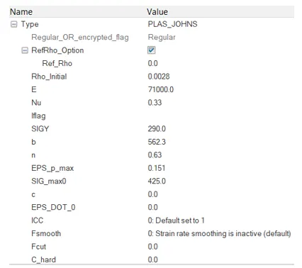
Default run is given to the model here and model has been saved under the name: Law2_epsmax_failure

Material Card(PLAS_JOHNS)

Material card name: Aluminum

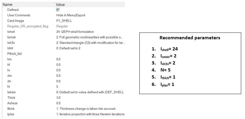
Property Card

Energy and Mass error, Simulation time, Total Number of cycles Case 1

Energy error= 0.8%(within 15%,therefore, acceptable)

Mass error= 0.00

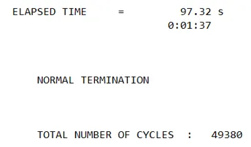
Simulation Time= 97.32 seconds

Total Number of cycles= 49380

Simulation Case 1

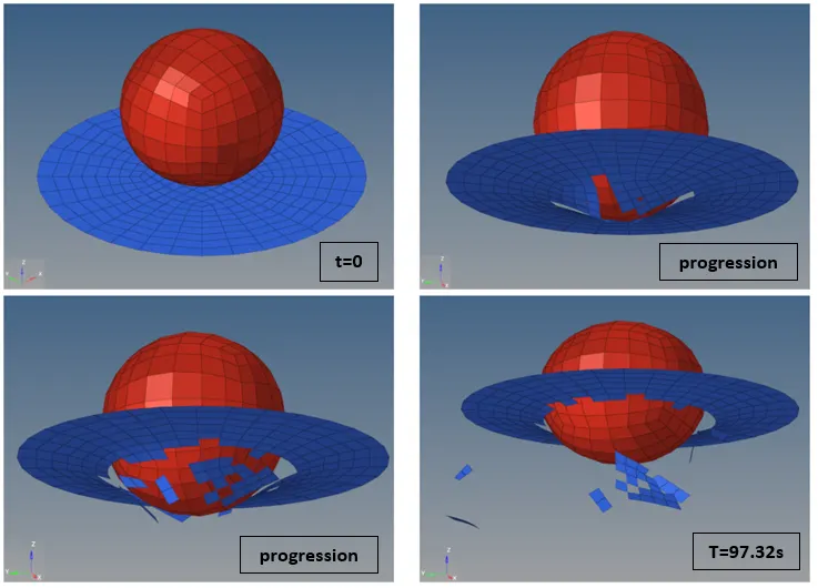
Contours and Plots (Case-1)

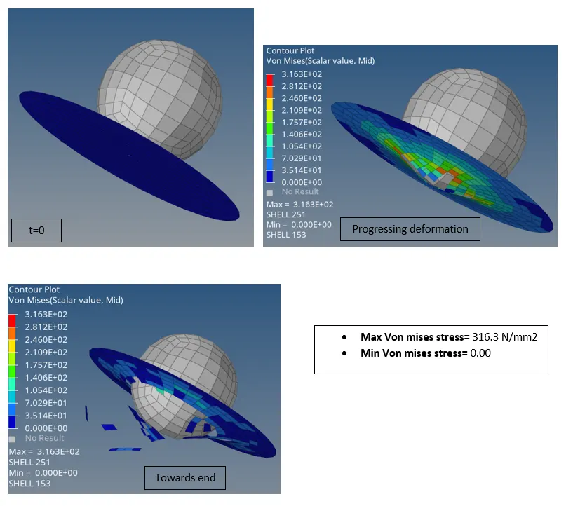
Von-Mises contour

Energy Plots

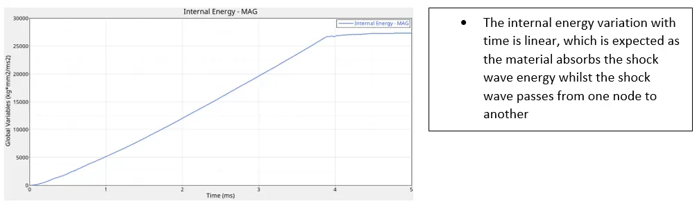
Internal energy

Kinetic energy

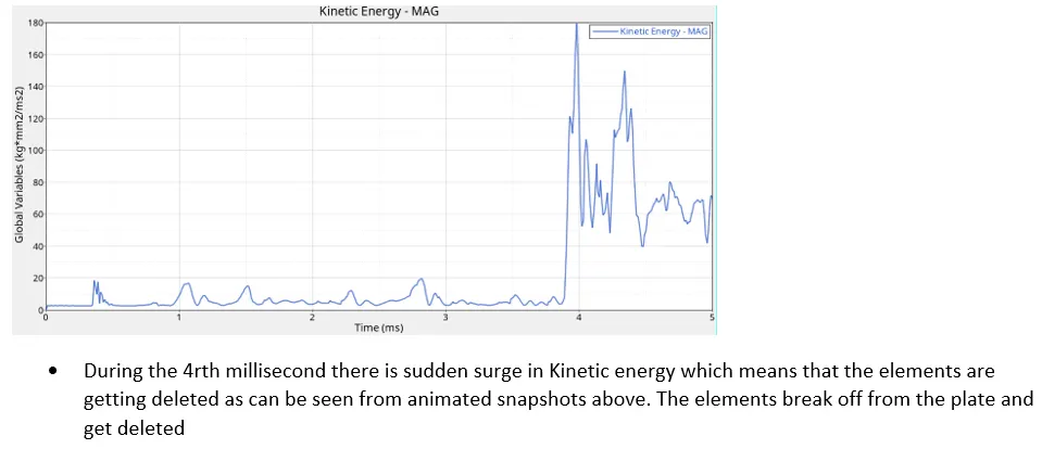
Final Kinetic energy= 67.81 units

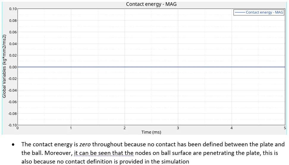
Contact energy

Hourglass energy

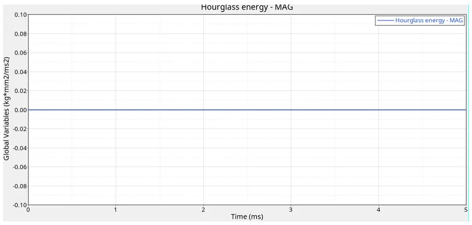
The hourglass energy is zero as the I_shell=24 elements are used i.e. basically, stiffness method is used in which the stiffness gets added at the material level only which takes care of most of the hourglass deformation even before they arise.

Case 2

Here, in /FAIL/JOHNSON the following values have been modified:

Ifail_sh= 1

D_adv= 1

I_xfem= 1 (To activate cracking of elements, to get a more realistic simulation)

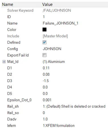
Energy and Mass error, Simulation time, Total Number of cycles Case 2

Energy error= 4.1%

Mass error= 0.00

This time the energy error came out to be higher than the previous case however it’s still within 15% limits which is the accepted benchmark.

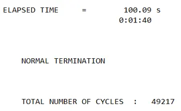
Simulation time(Elapsed time)= 100.09 seconds

Total Number of Cycles= 49217

The elapsed time this time is higher than the previous case as this simulation incorporated cracking up of elements too.

The total number of cycles however, in this case is lesser than the previous case.

Simulation Case 2

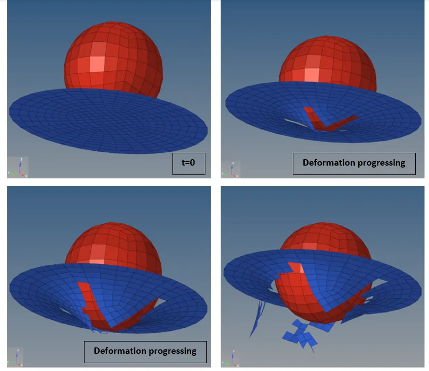
Contours & Plots Case 2

Von-Mises contour

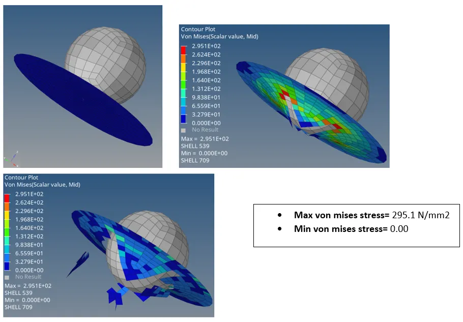
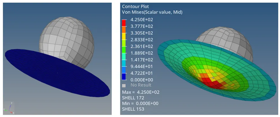
In this case, the maximum value of Von-Mises stress is less than the previous case i.e. less stresses have been generated in this case. This is implies, the material is safer compared to the case 1 material.

Energy Plots

Internal energy

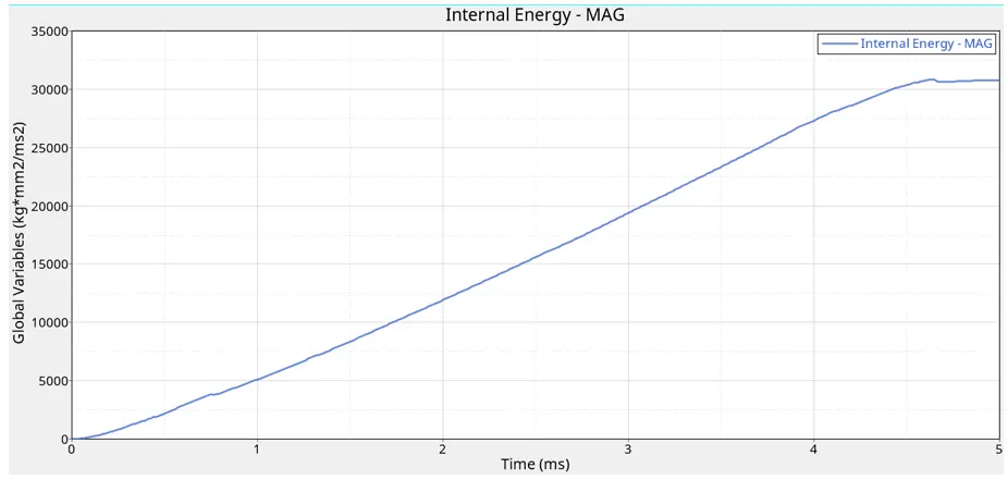
The internal energy has a linear variation as expected just like the previous case. It becomes flat after sometime indicating that fracture has occurred.

Kinetic energy

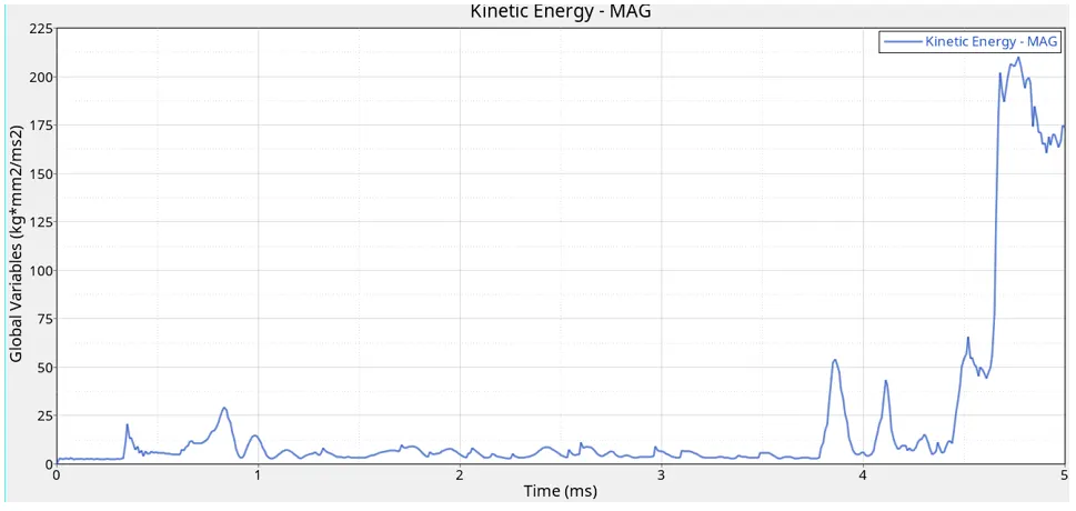
Final Kinetic energy= 141.9 units

It can be observed, Kinetic energy graph shows a spike slightly after 4.5^th millisecond as compared to the previous case where the spike was near the 4rth second. The element deletion process is delayed a bit in this case as the crack formation takes place here first due to the usage of Ixfem parameter.

Contact energy: It will be zero throughout as no contact definition has been given

Hourglass energy: This value will also be zero as “stiffness method” has been used as the hourglass control parameter which takes care of the hourglass deformation even before it starts at the material level

Case 3

Deleting /FAIL/JOHNSON card and running the simulation and file name is given as: Law2_epsmax_nofail

Energy and Mass error, Simulation time, Total Number of cycles Case 3

Energy Error= 0.8%

Mass Error= 0.00

0.8% is well acceptable limits of 15%

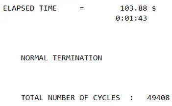
Elapsed time= 103.88 seconds

Total No. of cycles= 49408

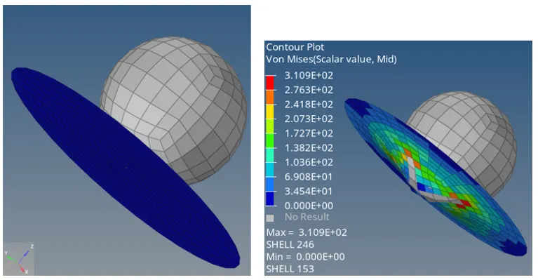
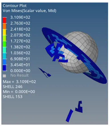
Simulation case 3

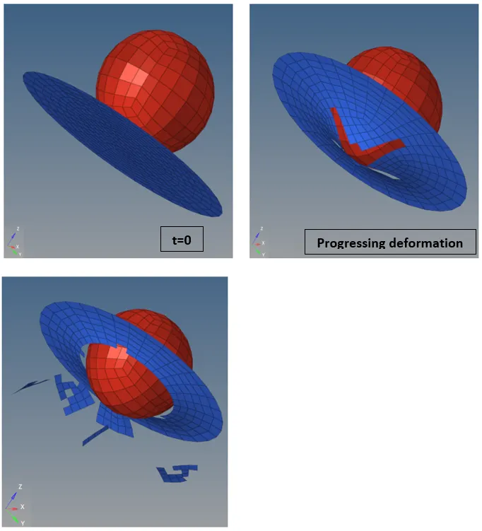
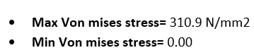
Von mises contour

Energy Plots

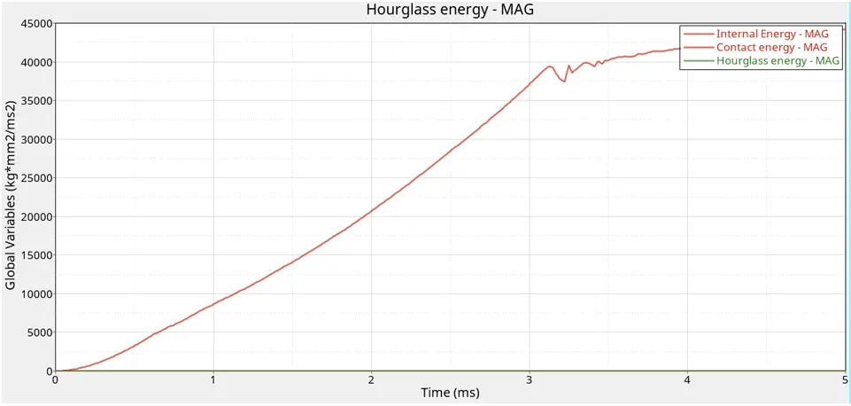
Internal energy, contact energy, hourglass energy

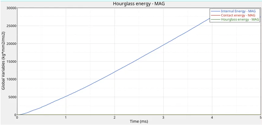
Again the variation of internal energy is as expected i.e. linear. The value of hourglass energy is zero as it is being taken care of by the element formulation selected. Also the contact energy is zero as no contact is defined. The internal energy curve flattens after the 4rth millisecond indicating fracture i.e. no energy is absorbed by material after fracture.

Kinetic energy

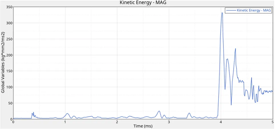
Final kinetic energy= 87.08 units

The surge before the 4rth millisecond takes place without a kink in this case as compared to Case 1 where there was a kink before the Kinetic energy reached it’s maximum value. The element deletion occurs superficially at the 4rth millisecond here.

Case 4

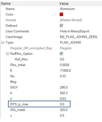
Deleting the value of EPS_p_max and running the model under the name: Law2

Modified Material property card

Energy and Mass error, Simulation time, Total Number of cycles Case 4

Energy error= 3.0%(higher than case 1&3 but lower than case 2, but within acceptable limits of 15%)

Mass error= 0.00

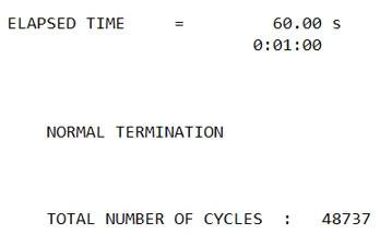
Simulation time= 60.00 seconds

Total No. of cycles= 48737

Simulation case 4

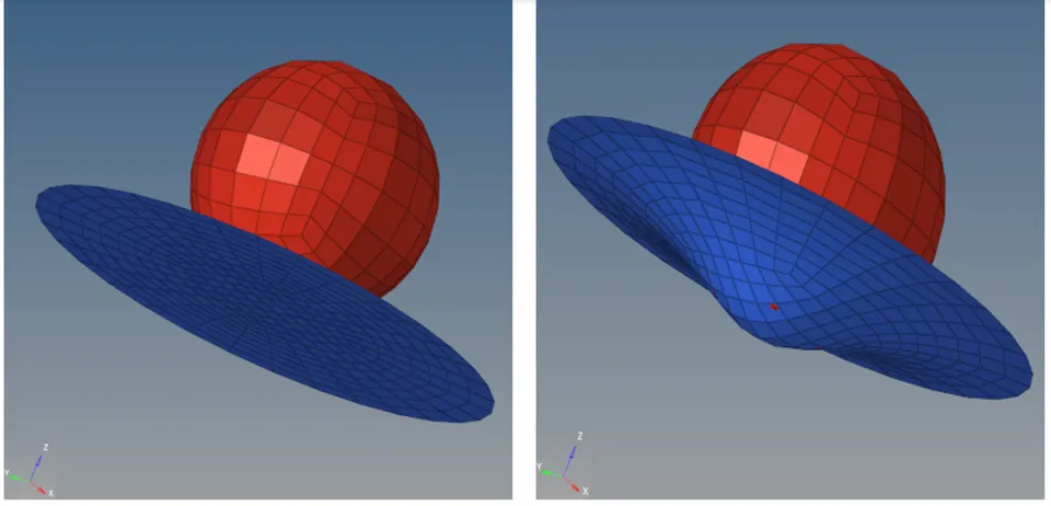
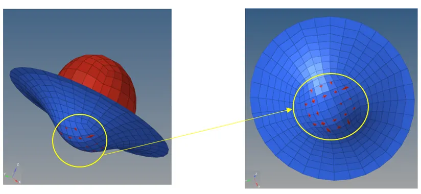
It can be construed from above graphic clearly that the nodes on the surface of the ball are passing through the plate surface which is because the contact between the ball and the plate is not defined. This case resembles the elastic case as the plate returns to it’s original shape after it has been unloaded.

Von-Mises contour

Energy Plots

Internal, contact, hourglass energy

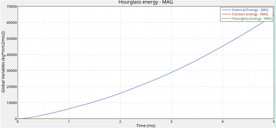
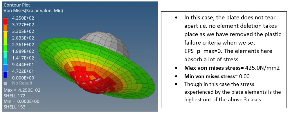
The internal energy in this case keeps on increasing linearly. The hourglass energy is still zero as QEPH element formulation is being used. The contact energy is zero. The internal energy here is higher than other cases, reason being there was no element deletion/failure criteria in this case, so the material absorbed a lot of energy as there was no limit specified.

Kinetic energy

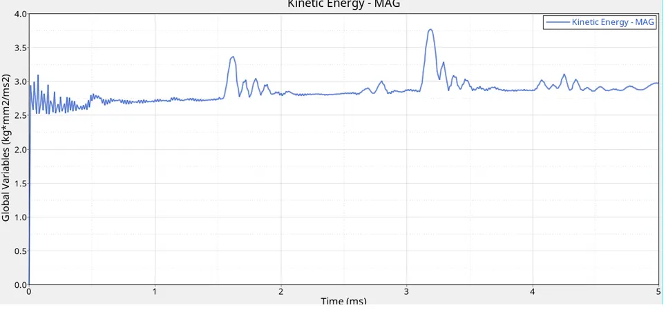
Final kinetic energy= 2.969 units

Since the elements were not getting deleted in this case, the kinetic energy has very less value compared to other cases where element deletion/failure was occurring. Maximum value being around 3.5kg*mm2/ms2.

Case 5

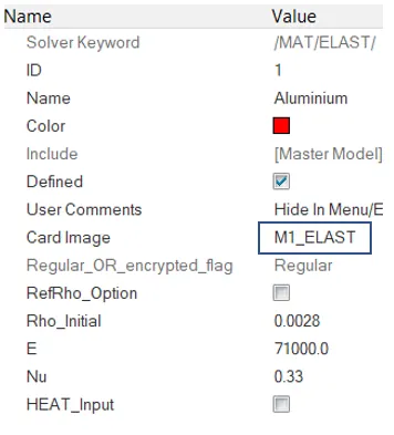
Converting current material model to LAW1 elastic with the same values of E, nu and density

Energy and Mass error, Simulation time, Total Number of cycles Case 5

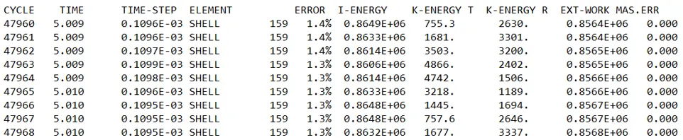
Energy error= 1.3%

Mass error= 0.00

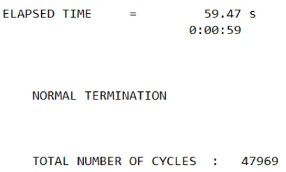
Simulation time= 59.47 seconds

Total No. of cycles= 47969

Simulation Case 5

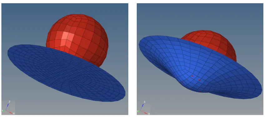
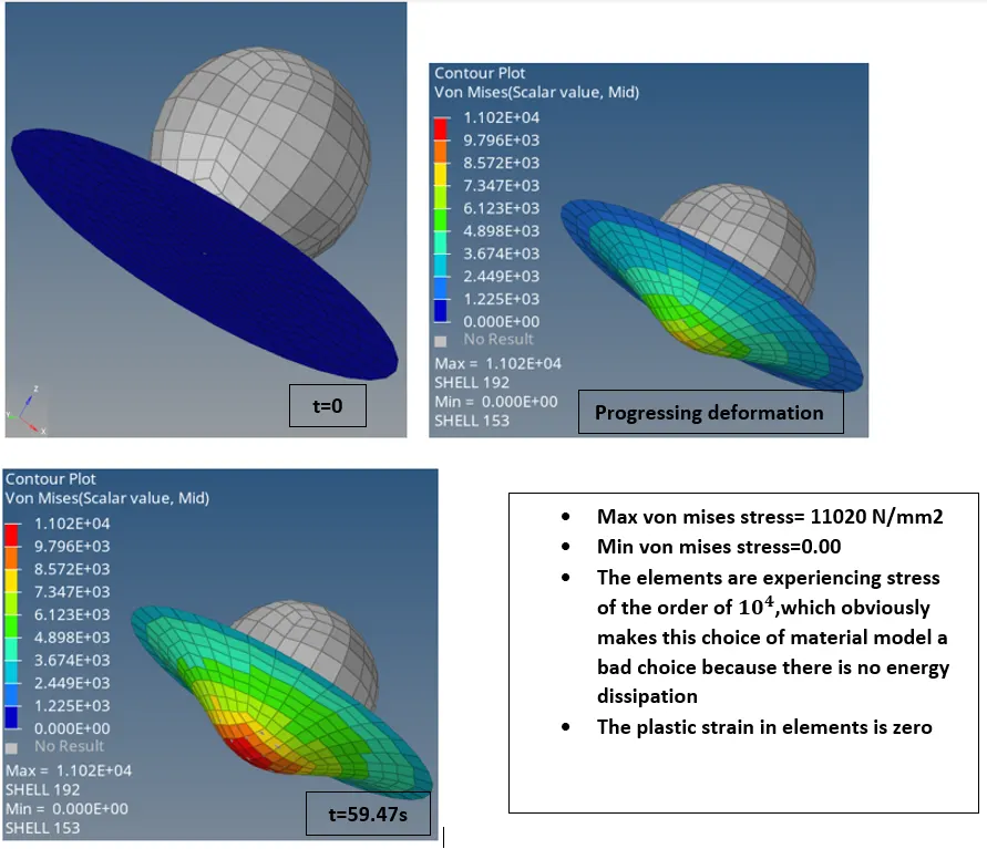
The elements are not getting deleted, as can be seen.

Von-Mises contour

Energy plots

Internal, contact, hourglass energy

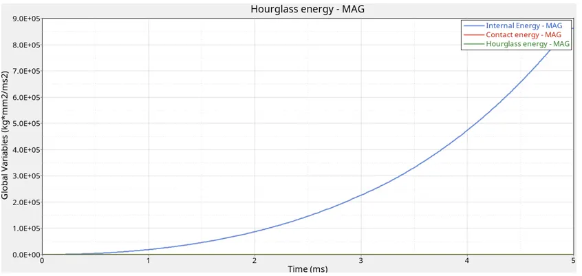
As can be seen, the internal energy in this case is very high as there is no set element failure/deletion criteria, they keep on absorbing large quantities of energy which results in high internal energy. The hourglass & contact energies are zero

Kinetic energy

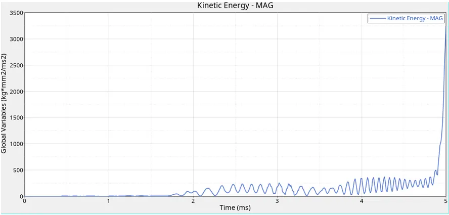
Final kinetic energy= 1677 units

The kinetic energy was low as no element were failing, had a surge at the end of simulation when deformation was highest.

Case 6

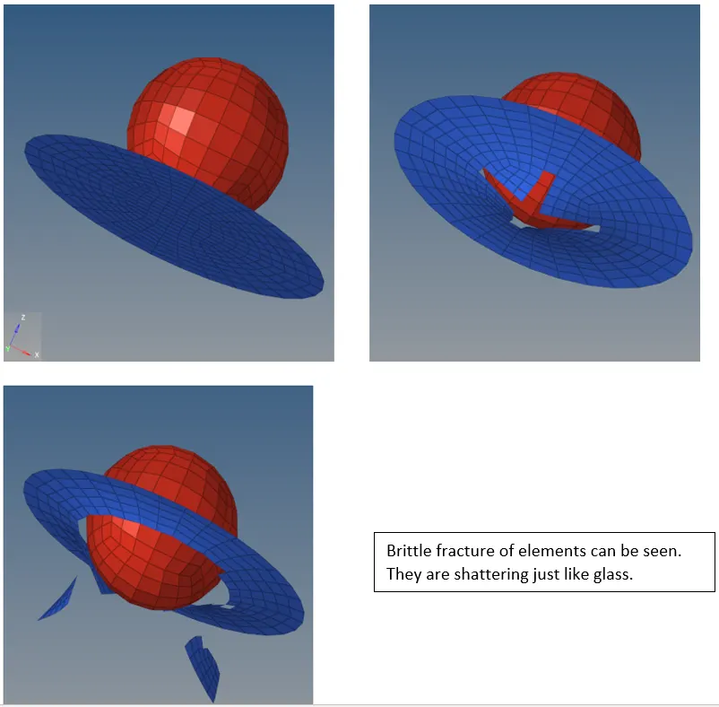
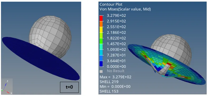
Working with the file: LAW27_000.rad

Simulation Case 6

Energy and Mass error, Simulation time, Total Number of cycles Case 6

Energy error= 0.8%(within 15% acceptable limit)

Mass error= 0.00

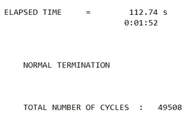
Simulation time= 112.74 seconds

Total No. of cycles= 49508

Von-Mises contour

Energy Plots

Internal, contact, hourglass energy

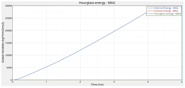
The Internal energy rises linearly while the contact and hourglass energies remain zero throughout.

Kinetic energy

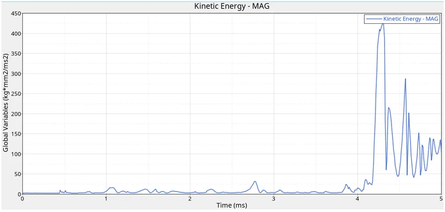
Final kinetic energy= 65.0 units

A surge in the kinetic energy can be seen around the 4.25^th second of the simulation where the elements fail and get deleted.

Case 7

Workability with LAW36

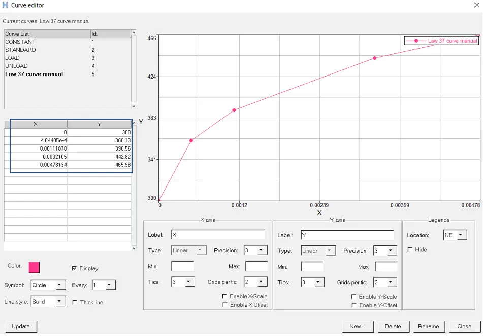
X and corresponding y values have been obtained from the lab

A new curve is created with the name: Law36 Test Curve with the following parameters:

The material and property card as follows:

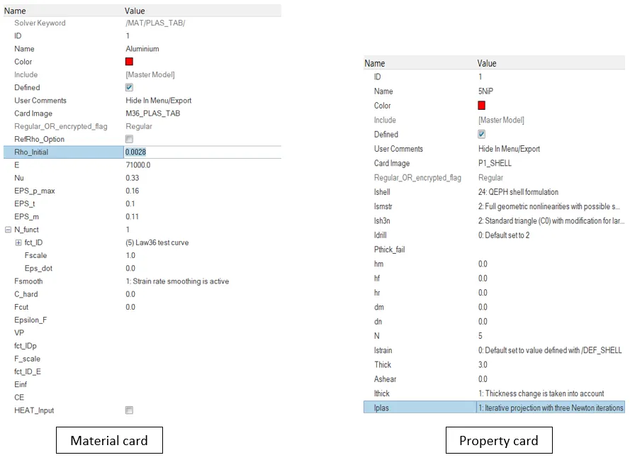
The energy error is well within acceptable limits

Simulation Case 7

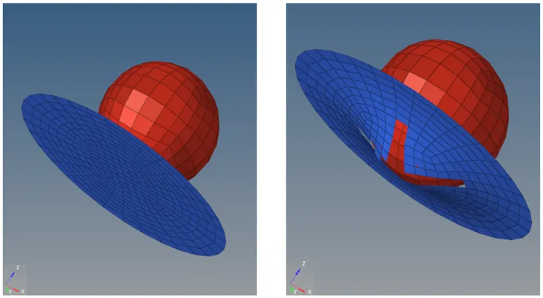
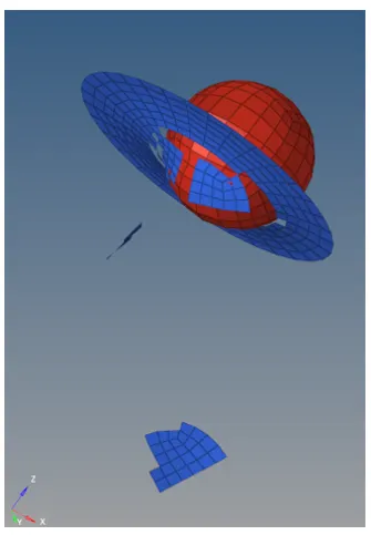
Von-Mises contour

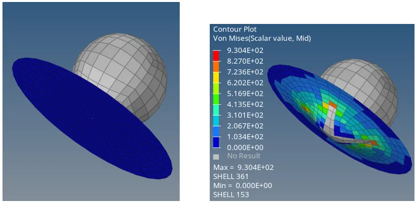
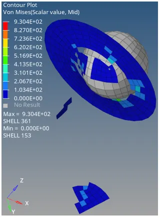
1. Max von mises stress= 930.4 N/mm2
2. Min von mises stress= 00
3. The stress experienced by the elements in this case is also extremely high

Energy plots

Internal, contact, hourglass energy

Kinetic energy

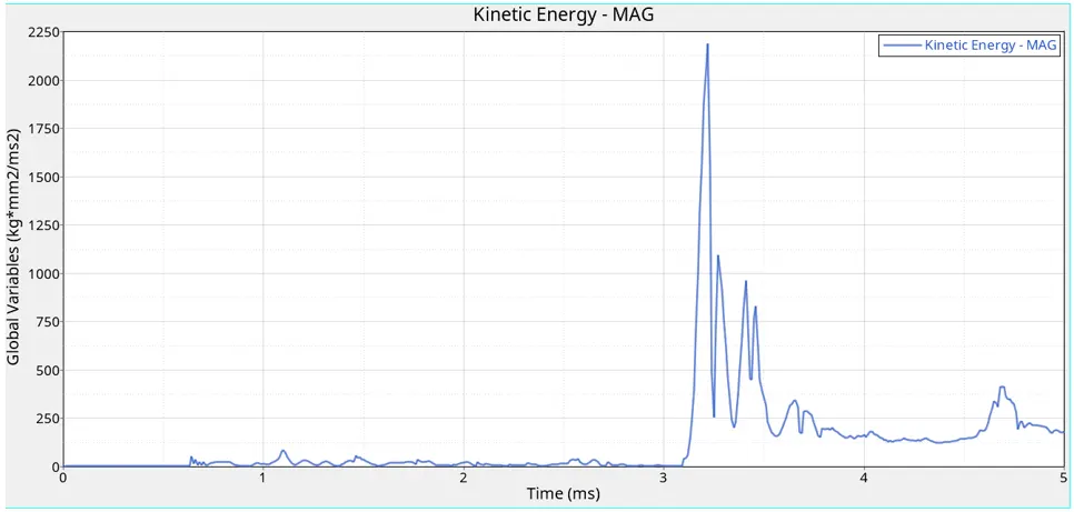
Final kinetic energy= 177.7 units

A sudden surge of kinetic energy can be seen around 3.35^th millisecond

Result Comparison of 7 cases

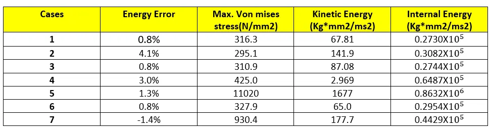
1. The hourglass & contact energy in all cases is zero The hourglass is being taken care of by the QEPH element formulation(stiffness method). The contact energy is zero as no contact has been defined.
2. Case 2 is preferred because the elements experience less von mises stress in this case compared to others. Also in this case, Ixfem is set to 1 which helps in realizing the crack formation in the elements more clearly compared to when they get deleted directly from the system.

Conclusion

Successfully simulated and compared the results for different materials applied to rupture plate, observed the crack formation, element deletion on specified failure criteria.