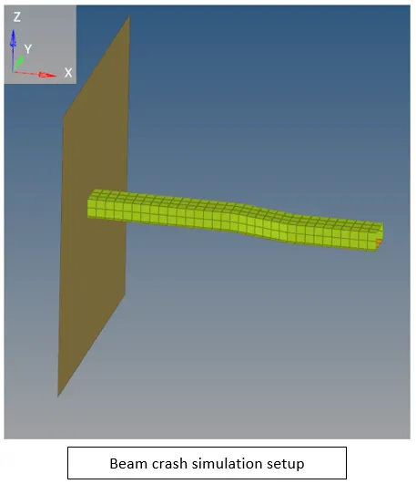
To run the crash beam simulation with and without modification to element properties and comparing the results of the two case setups
Aim: To run the base simulation of crash beam with and without modification to element properties and comparing the resultant plots of the two case setups
Objective of project:
- To carry out base and modified element properties simulation
- To check energy and mass errors and decide whether results are acceptable
- To compare the plots of rigid wall forces, internal energy, hourglass energy, contact energy, total energy of the two simulation setups
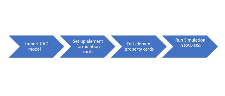
Workflow
Theoretical Aspects
2D shell mesh importance and use
Shell elements are used to model structural elements in which two dimensions are much greater than the third one and when the change of the analyzed feature across this third direction can be neglected
- Used for extremely thin features(t<=6mm) or in general, if the thickness of the body is at least 20 times less than the span
- Easy to create
- Less problems with stability
- Needs much less disk space for results
- Faster post-processing
Shell element time step
The formula for the time step is straight forward, `deltat=l/c`
`deltat= time step`
l:critical length
c:speed of sound through the material
Note: Critical length is usually the minimum height of the element
The critical length can vary with the following:
- Shell formulation
- Hourglass control parameters(discussed ahead)
- Numerical damping
- Membrane damping
Shell Element Formulation
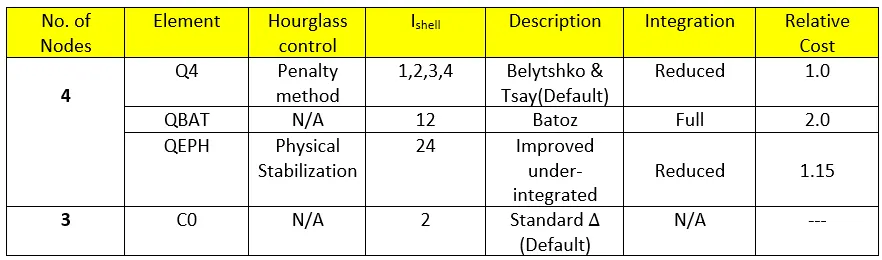
- RADIOSS provides both reduced and fully integrated 4-noded shell elements
- 3-noded shell element is also available in RADIOSS
Reduced integration schemes have 1 integration point on the surface. It is widely used in programs with explicit time integration applied in Crashworthiness studies. This scheme type also dramatically reduces the computation time compared to 4- point integration but is somewhat less accurate. It is a competitive scheme if the hourglass modes(which result from reduced integration schemes) are well stabilized.
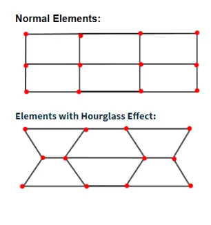
Hourglass: It is a condition in which a node is moving/displaced but it is not recording any stress which is a bad situation because if it’s not recording any stress then that stress won’t develop any forces in the rest of the nodes and that will simply break off the time step cycle
Key Parameters in /PROP/SHELL
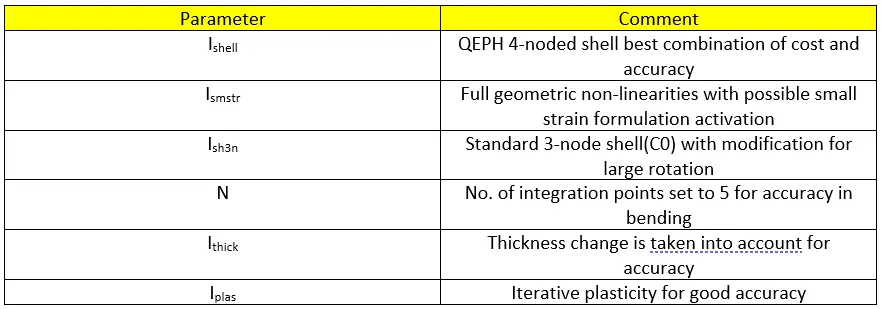
- Ishell: To select element formulation for 4-noded shells
- Ish3n: To select element formulation for 3-noded shells
- N: To choose number of integration points through the thickness(discussed ahead)
- Ismstr: To specify small or large strain formulation(discussed ahead)
- Iplas: To choose method for calculating post-yield strains(discussed ahead)
- Ithick: Determine if thickness is constant under load, or if thickness varies(discussed ahead)
Note: The gauss integration points help us with the hourglass problems whereas the thickness based integration points(N) help us with the accuracy of the results.
- QBAT is not economical compared to Ishell=1,2,3,4 but it is the most accurate because it involves a great number of gauss integration points to calculate nodal values
- In QEPH(Ishell=24) though it is under-integrated there is an improvement because it has physical hourglass stabilization(stiffness method)
- QEPH is an improved under-integrated 4 node element with 1 integration point on the surface. It is the best compromise between cost and accuracy. Generally, the QEPH elements cost 15% more than Belytshko &Tsay element but the results are in propensity of QBAT type
Hourglass due to Reduced Time step
1. Hourglass modes are non-physical modes of deformation that occur in under-integrated elements and produce no stress.
Note: Under-integrated means: either there is a solid element with a single integration point or a shell or Tshell elements with a single in-plane integration point
2. Reduced integration can lead to non-physical zero energy models, called hourglass models
3. There are two methods to control formulation of hourglassing, namely:Perturbation(Q4 elements)
- Physical stabilization(QEPH elements)
Hourglass Control Methods
- Hourglass Perturbation control method:
Also known as Perturbation(viscous) methos (for Ishell= 1,2,3,4 i.e. Q4)
In this case, it adds a damping to the node and that nodal damping is going to add stiffness externally.
- The hourglass deformation is detected with the relative motion of the nodes
- When hourglassing is detected, a force is applied on the node to stabilize the deformation
- This force is defined according to element stiffness
- This force induces an artificial energy called hourglass energy
2. Stiffness Method (Ishell= 24)
In this case, the stiffness is artificially added on the element and thus, it affects the material property directly
- Hourglass yield depends on natural yield
- Hourglass loading stiffness depends on natural tangent modulus
- The hourglass treatment is done at the material level
Note: The stiffness method is generally preferred more because the stiffness is added at the material level itself. So most of the hourglasses are getting controlled even before they arise that is why there is less need for the hourglass energy to be used to control those hourglass deformation. While, in viscous method the damping is going to be applied only when the software is trying to detect the deformation of hourglass type, there is a good chance that there will be huge amount of artificial energy getting generated(hourglass energy). The basic point being, stiffness method causes less energy to be spent in hourglass.
Hourglass Control Method Comparison
- The Q4 elements may have spurious behavior in case of large rotation and distortion problems and in case of elastic loading-unloading cycles. The viscous method inhibits additional hourglassing deformation(it can’t recover from previously accumulated Hourglass deformation). It is preferred for hi9gh velocity/high strain problems e.g. Those involving explosives
- The QEPH elements give accurate results in case of loading and unloading and even if there is hourglass mode deformation. This method is able to reduce total accumulated hourglassing deformation. It is preferred for lower rate problems, including crash simulation
Shell Stress Computation
- From the deformation and strain rates, RADIOSS computes the strain at each integration point
- Using this strain, the stress is computed with an elastic increment
- With the computed stress values the von-mises stress is calculated and compared to the yield stress of the material
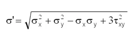
- If the von-mises stress is smaller than the yield stress, the computed is the one used in order to compute the internal force of the elements
N(Integration points)

- N=5 integration points is recommended because it keeps one integration point on the surface of the 2D element and then there are two integration points on either side of the shell element
Ismstr

- Small strain: Usually for problems with small deformation, strain is computed based on the initial element size
- Large strain: For problems with large displacements and strains, strain is computed based on current element size
Iplas

- Iplas gets activated in the solver as soon as the stress value reaches the yield stress value, because beyond there onset of plastic deformation
- When the we are in the elastic region, the thickness more or less remains constant but, when we enter the plastic region i.e. the stress value exceeds the yield stress value of the material, the shell elements somewhat distorts i.e. it’s thickness changes
Ithick

- Initial thickness is used to compute strains & to integrate stresses, but the thickness variation is still computed for post processing reasons
- If a variable thickness is used, true thickness is computed both for post-processing and for strain computation
- In cases of necking or spring back, it is advisable to use iterative plastic projection and thickness variation
Shell Elements Formulation used
Energy Error:
- The error must be negative and decreasing. The error must be less than 15% at the end of computation(5% recommended)
- Ideally, the error at most should be -15% and better to have -5%. The closer to 0%, the better
- An error of 1% or 2% is acceptable otherwise any positive energy error means energy has been created, which is obviously not possible and it indicates a model issue
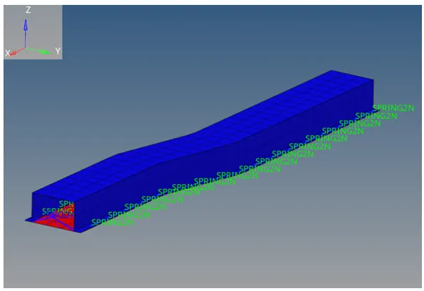
Model Provided
Simulation 1 Details
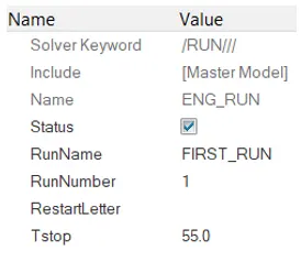
- Editing ENG_RUN
As per requirement we set Tstop= 55ms
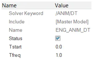
- Editing ENG_ANIM_DT
Here we have taken 55 animation steps for which,
Tfreq=1.0
- For the first simulation the element formulation properties are referring to default card values i.e. the values already set in /DEF_SHELL
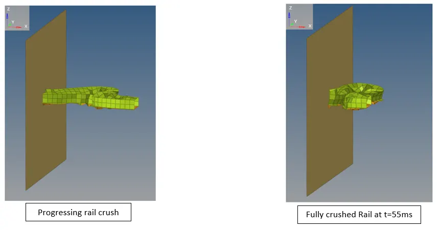
Energy & Mass Error checks(Simulation-1)
For checking Errors, we refer notepad file: FIRST_RUN_0001.OUT
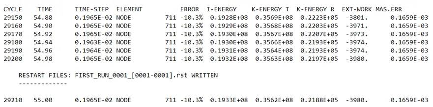
From above snapshot we can see that at the end of simulation i.e. t=55ms:
- Energy Error= -10.3%
- Mass Error= `0.1659X10^-3`
Energy error is within -15% which is acceptable to a limit, but this can be improved as discussed further
Contours
Displacement contour
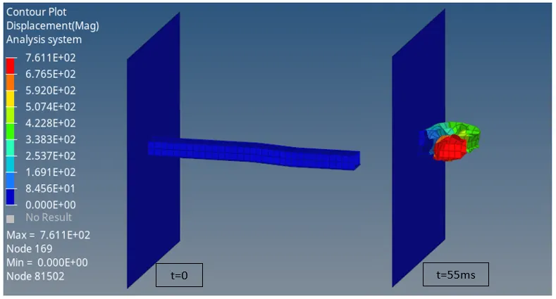
- Max Displacement= `7.611X10^02`mm
- Min Displacement= 0mm
Von-Mises Contour
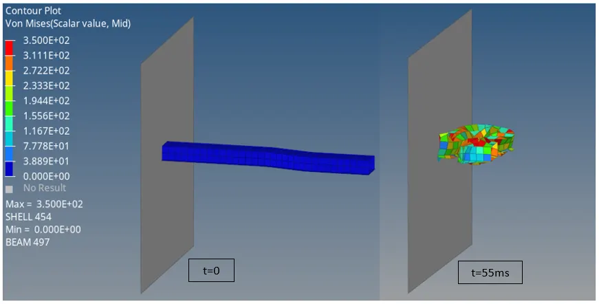
- Max Von-Mises stress= `3.5X10^2`N/mm2
- Min Von-Mises stress= 0
Plots
Rigid wall forces vs Time
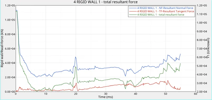
- In the beginning, the reaction force from the wall is maximum and gradually during the crash it decreases because the material absorbs the energy as the shock wave moves from element to element.
- It can also be seen that the force values as the time progresses is quite erratic
Energy plots
- The following plot incorporates the various energy types namely: internal energy, Kinetic energy, contact energy, Hourglass energy, Total energy(TE) vs time
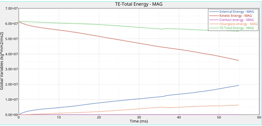
- The kinetic energy in the beginning is maximum and gradually decreases as the speed decreases during the crash with wall
- Hourglass is increasing due to the hourglass deformation
- Internal increases as the material absorbs the energy from shock wave
- Overall, total energy is decreasing
Simulation 2 Details
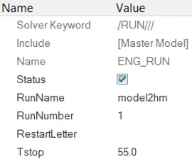
- The ENG_RUN card is set as follows:
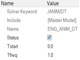
- ENG_ANIM_DT is set as follows:
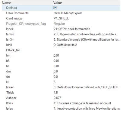
- The property cards of Hat-section & Close-out panel are edited as follows:
Energy & Mass Error checks(Simulation-2)
For checking Errors, we refer notepad file: model2hm_0001.OUT

From above snapshot we can see that at the end of simulation i.e. t=55ms:
- Energy Error= -0.1%
- Mass Error= `0.1659X10^-03`
Energy error is very close to 0%, the closer to 0% the better
Contours
Displacement contour
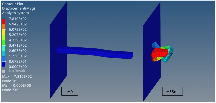
- Max Displacement= `7.81X10^02`mm at t=55ms
- Min Displacement= 0mm at t=0
Von-Mises Contour
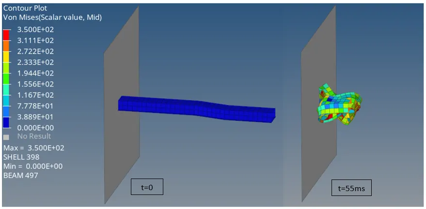
- Max Von-Mises stress= `3.5X10^2`N/mm2
- Min Von-Mises stress= 0
Plots
Rigid wall forces vs Time
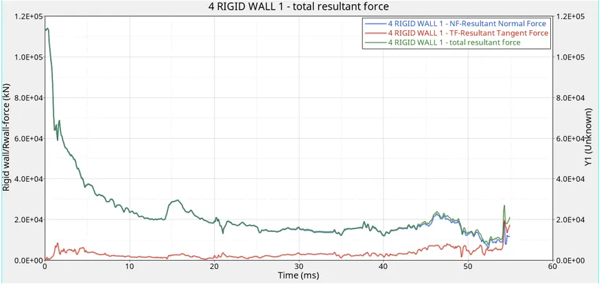
- During the onset of crash i.e. at t=0 the Reaction force from the wall is maximum and it gradually decreases as the material absorbs the shock wave energy. This modified simulation’s rigid wall force plot seems to decrease more uniformly than the previous simulation settings(refer simulation-1 plot)
- The force values as the time progresses is not as erratic as the previous simulation
Energy plots
- The following plot incorporates the various energy types namely: internal energy, Kinetic energy, contact energy, Hourglass energy, Total energy(TE) vs time .
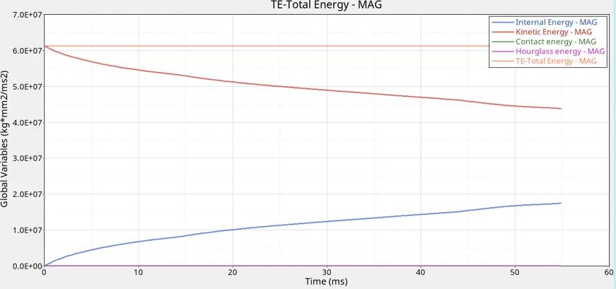
- In this case, the hourglass deformation is ZERO due to which hourglass energy is also zero
Result Comparison of Simulation 1 & 2
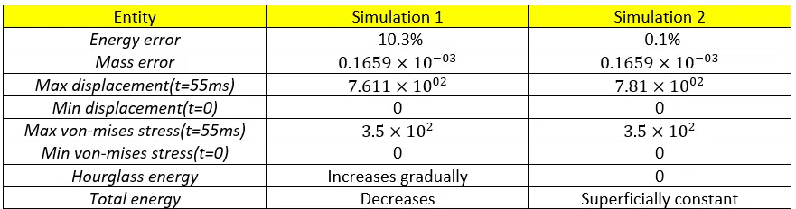
Unit system: Kg mm ms
The change in the displacement values in the two cases can be explained by the fact that the element properties were modified in the second case to better type elements where Ishell=24(QEPH) which is a good compromise between cost and accuracy and also Ismstr=2 which incorporates Large strain with full geometric non-linearitiesUnit system: Kg mm ms
- The value for Ithick for both simulations are same i.e. 1 in which thickness change is taken into account for better accuracy
- Iplas=1 in both simulation cases for good accuracy
- N=5 for better bending accuracy
- Internal energy in both the cases increases as the material absorbs the shock wave
Conclusion
- Successfully carried out base simulation and modified simulation with the changed element properties
- Compared results: energy, rigid wall forces and von-mises stress obtained in the two cases