Analysis of failure behaviour of plates using law-1,law-27,law-36 material models and johnson cook failure card in Radioss

OBJECTIVE:

To analyze the plate failure behavior using different material models

THEORY:

In FEA non-linear simulation, material modeling is a very complex step where you need to capture the plasticity of the material accurately and its failure. This experiment will use model with different material laws like LAW-1 Elastic, Law-2 Elasto-plastic, LAW-27 Brittle, and LAW-36 Elastoplastic to understand the modeling techniques and their failure with a Johncock failure card. We will also use the XFEM failure formulation to understand the crack propagation effect in brittle materials. For all the above experiments Aluminium is taken as the material

MATERIAL PROPERTIES:

Initial density(`rho`)=0.0028 g/mm3

Youngs Modulus(E)= 71000MPa

Poissons Ration(nu)=0.33

True Yield Stress (a)= 290MPa

Hardening Modulus or UTS(b)= 562.3

Hardening exponent(n)=0.63

Maximum plastic strain for failure(EPS_p_max)=0.151

Maximum stress(sig_max0)=425Mpa

PROCEDURE:

CASE I: Simulate with both failure plastic strain and failure Johson card

1. Import the given model in hypermesh

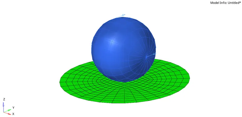
2. Checkout the solver deck cards and properties.

Here Eps_p_max=0.151 hence the elements will fail when it reaches 15% of the plastic strain

Xfem=0-Elements are deleted when it reaches 15% of the plastic strain value

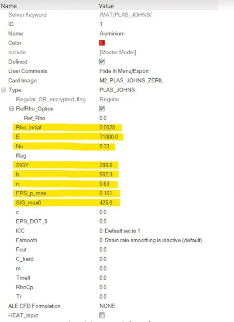
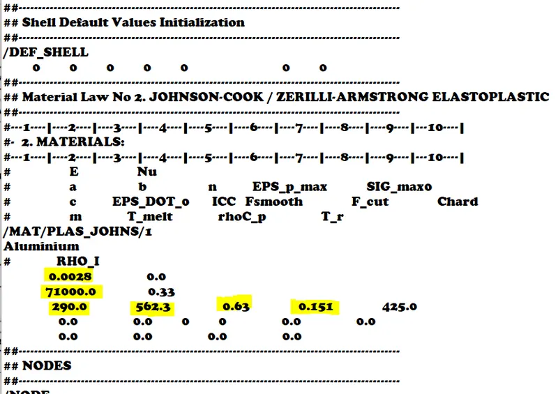
Material card in RADIOSS Material Block in Starter input file

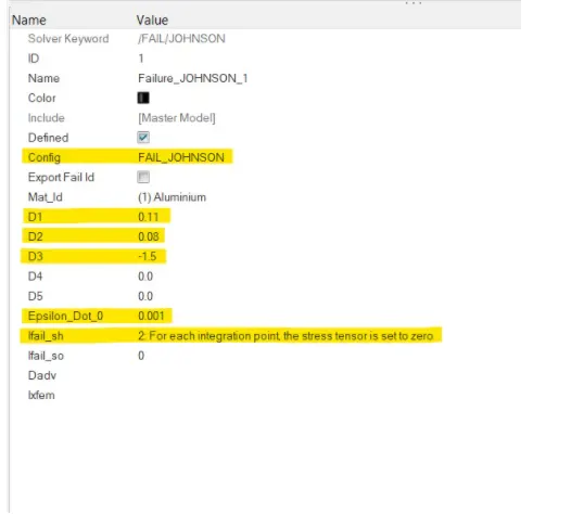
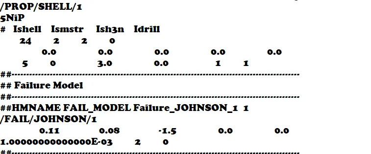
Failure card in RADIOSS Failure model block in starter file

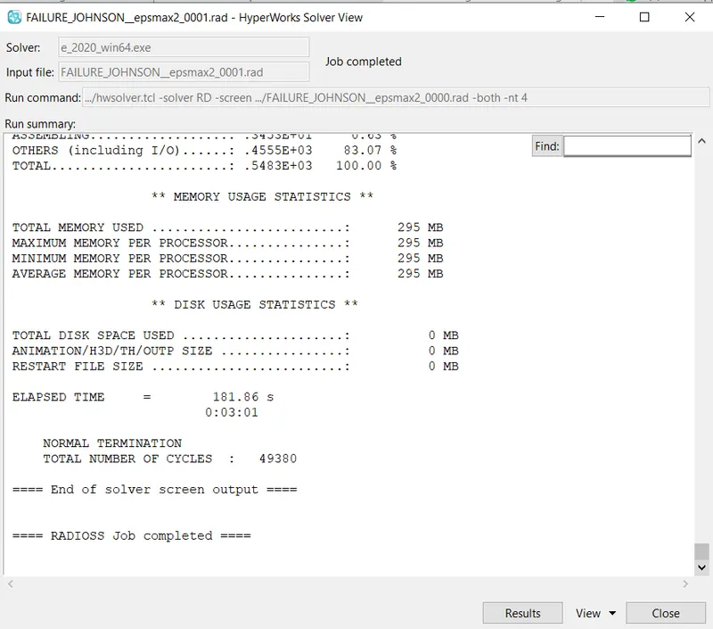
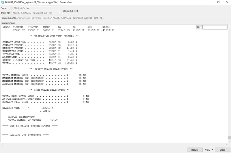
3.We have to run the analysis with the made changes. Go to the Analysis-->RADIOSS option save the file and run the analysis. We get a Hyperorks window opped out after completion of the work

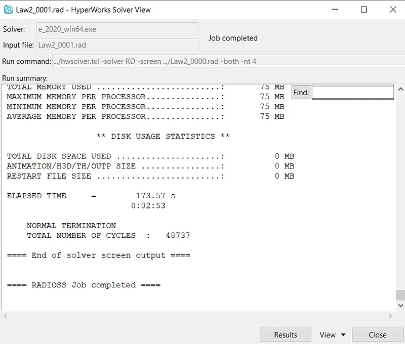
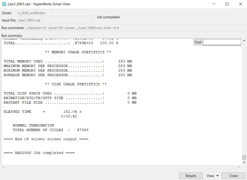
We set the options panel to -nt 4 for faster computation of the results. From the below window we get know the total no of cycle and time taken for the computation of the results

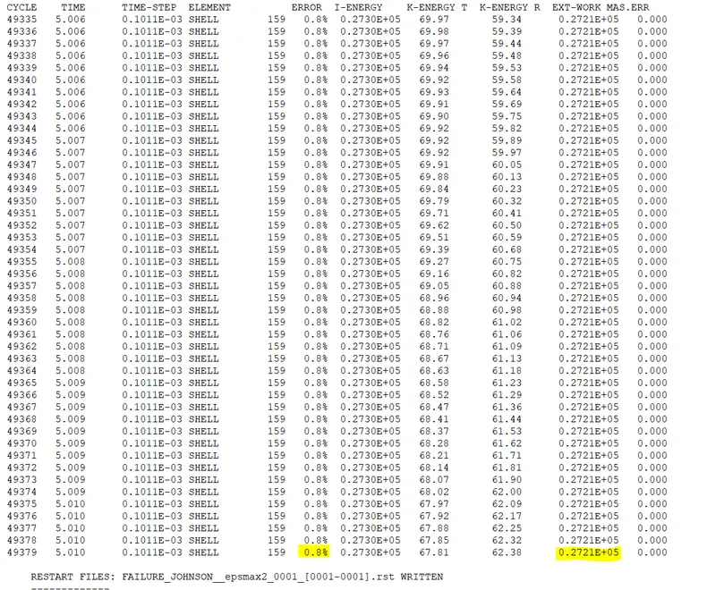
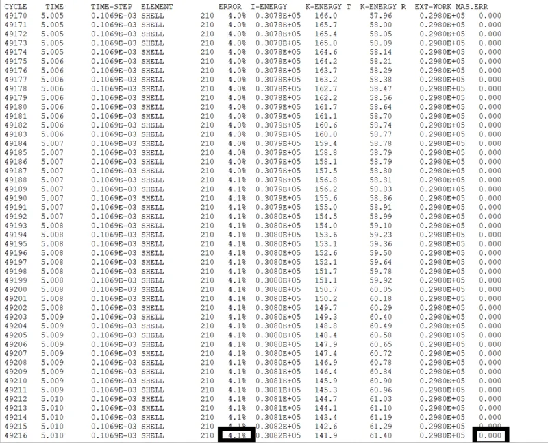
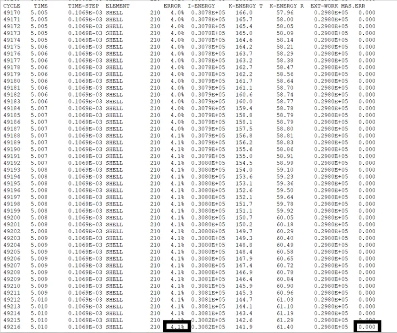
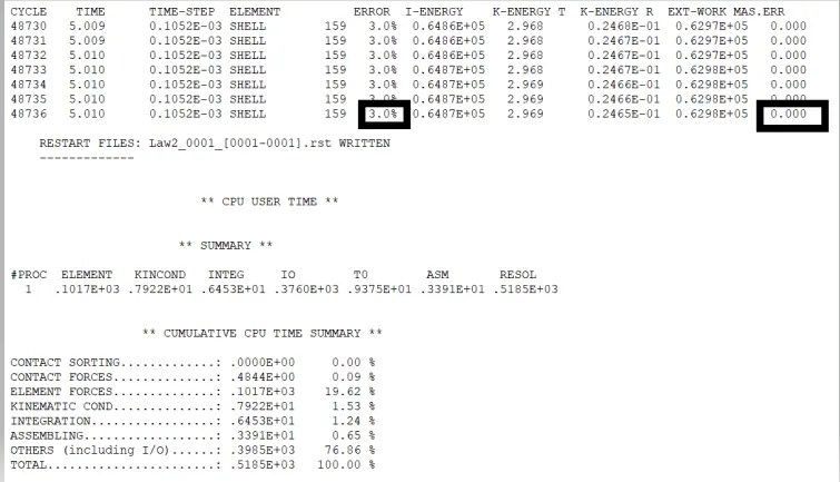
4. After successful completion of the run open the radioss engine out file and check for errors. Mass error should lie within (2-3%)and energy error should lie within (5 to -15%).We find that errors are well within the range. Hence here the results are acceptable. Now we move forward for post-processing of the results

5. Now we go for the post processing stage.First we open the animation(.h3d file) in hyperview post-processor. We create the necessary contours required for the study and later move on to hypergraph for plotting the required data

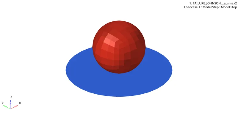
Post-processing the results through Hyperview

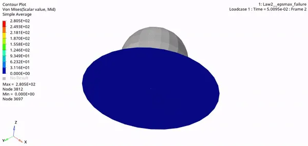
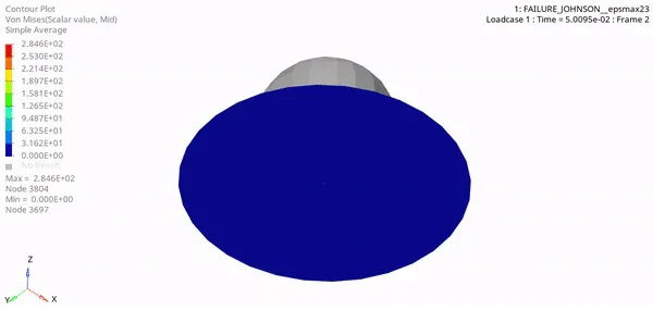
Von-mises stress contour

6.Next we open hypergragh to plot our required data. We open the T01 file type in hypergraph and select our required values to plot the graph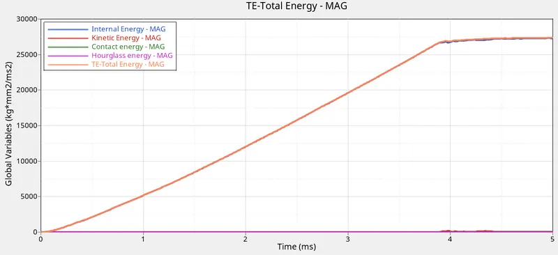

Time vs IE_KE_CE_HE_TE

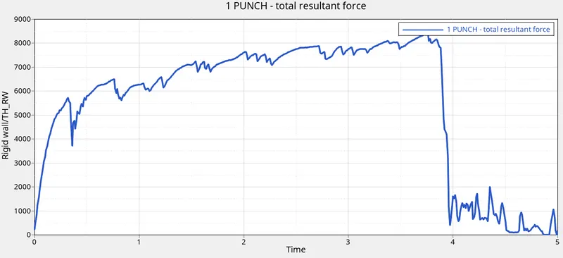
Time vs Resultant force(N) on the rigid sphere

i.In case case 1 we have both the Eps_p_max as well as the fail johnson failure model defined.Fail_johnson is a ductile type failure model used in case of ductile metals,mostly while using material Law2(Johnson cook material mode) for the components.

ii.The fail_johnson failure model calculated the failure plastic strain using 5 parameters,D1,D2,D3,D4,D5.How the failure happens is decided by the lxfem value. A value of 0 will lead to the failed element getting deleted and a value of 1 will cause the element to fail by crack propogation.In latter case the crack advancement is decided by Dadv value which can vary from 0 to 1.

iii.For this particular simulation we can see that the elements have failed by element deletion as lxfem was defined as 0. We also observe that Von-mises stress contour animation the maximum stress was just before the rigid ball punched a hole in the plate ~4m/s

II.Case 2: Simulate with failure plastic strain(Eps_p_max) and fail_johnson failure car enabled [lshell=1,Dadv=1,lxfem=1]

Change the respective values in the failure card as necessary.lshell_sh is the shell failure flag.Its default value is 1.It decides whether the failed elements are to be deleted or cracked.

Dadv -->Gives the criterion for crack advancement[Only active when lxfem values is set as 1]

Ifail_sh=1-->Elements will get deleted when the stress reaches one integration point

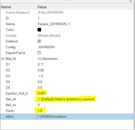
We have to run the analysis with the made changes. Go to the Analysis-->RADIOSS option save the file and run the analysis. We get a Hyperorks window opped out after completion of the work

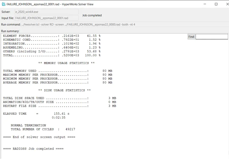
After successful completion of the run ,we open the radioss engine out file and check for errors. Mass error should lie within (2-3%)and energy error should lie within 5 to -15%.We find that errors are well within the range. Hence here the results are acceptable

Now we next move for post-processing the results.We use hyperview and hypergraph to get the necessary contours and plots

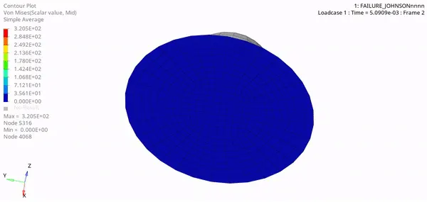
Von-mises stress contour

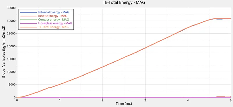
Time vs IE_KE_CE_HE_TE

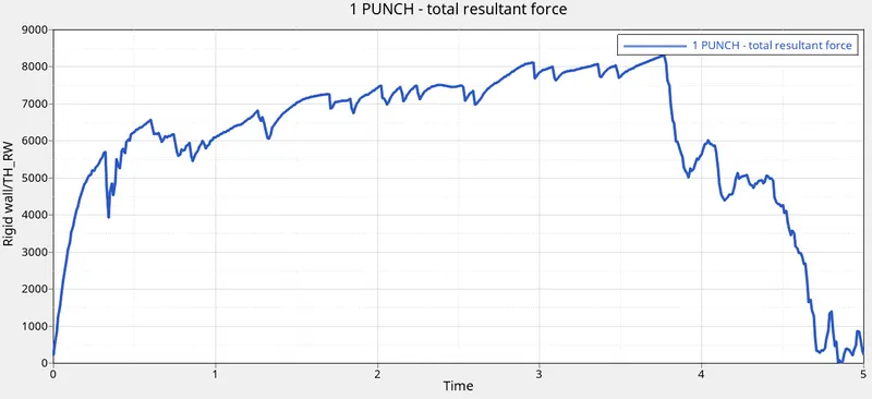
Time vs Resultant force(N) on the rigid sphere

i.In case 2 , we have changed the lxfem value to 1 and therefore the elements are failing by crack propogation.Here the elements are not getting deleted right away but getting cracked on reaching the failure strain value

ii.The time vs energy plots clearly shows a delay in element deletion.Here unlike the previous case the dip in iinternal energy is observed at ~4.6m/s. Here the energy is dissapated through the cracks

iii.This can be exlained by the fact that unlike case 1, the elements did not completely get deleted.Instead ,cracks ere developed.Also less number of elements have comparitevely broken off

III CASE 3: Now we delete the johnson_failure card and proceed for simulation

Repeat all the previous steps and run the analysis.Analysis-->Radioss-->save as-->Radioss

Now we next move for post-processing the results.We use hyperview and hypergraph to get the necessary contours and plots

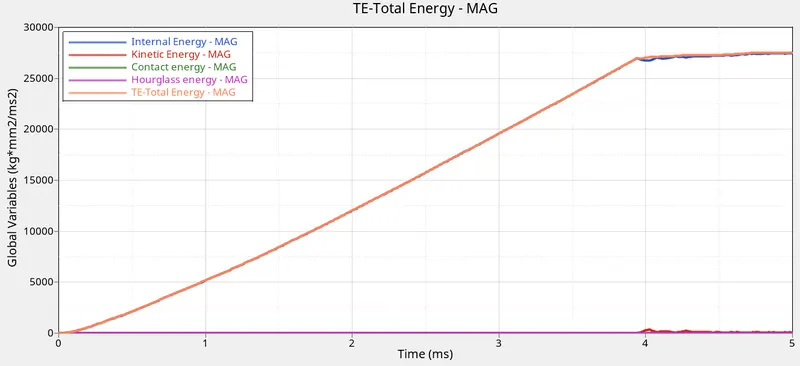
Time vs IE_KE_CE_HE_TE

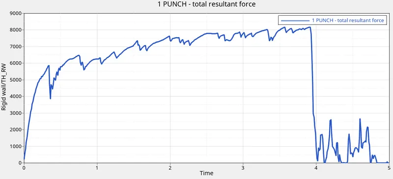
Time vs Resultant force(N) on the rigid sphere

i. Here in case 3 the deletion mod was the failure model.Elements going to fail depends upon the Eps_p_max value defined in the material card,which in this case happens to be 0.151 or 15% of the plastic strain.

ii.The time vs energy plots indicate the steady rise in total energy and internal energy untill the point in the simulation where elements get broken

iii. The time vs Resultant force plot shows a steep incrase in those forces at the beginning and as the elements begin to fail and gets deleted the plot begins to fluctuate.The dip indicates deletion of new elements

IV. CASE 4:The model has no eps_max and failure card.

Import the given model in solver deck

Here we move without both eps_max and johnson failure.Hence we delete it and proceed with the simulation.

Repeat the steps from case 1

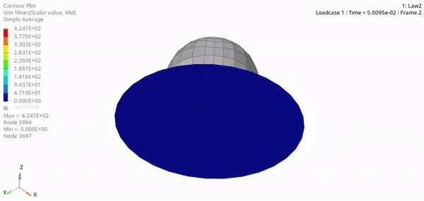
Von-mises stress contour

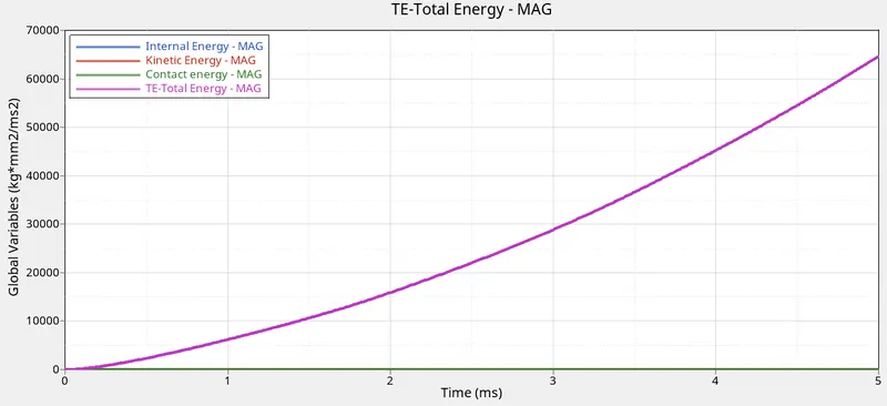
Time vs IE_KE_CE_HE_TE

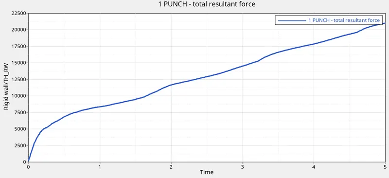
Time vs Resultant force(N) on the rigid sphere

i. In case 4 the Eps_p_max value also has been removed.Thus there are no failure parameters defined for the plate

ii. The energy plots have recorded a nonlinear increase in both IE and TE whereas KE & HGE have remained zero throughout the simulation

iii.Here the forces on the rigid sphere are seen to have continuously increased all throughout the simulation

V. Case 5:Simulate after changing the material law to law 1

Import the given model in the solver deck

Go through the solver deck cards and properties

Change the material law to law 1 which for elastic materials.As these material follow elastic property they expand as the load keep on increasing and return back to its original shape.Its preferable for parts that will never cross the yield limit but in applications like crash analysis its not suitable.

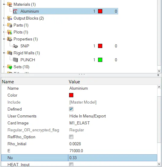
After setting up the properties we now move on to the analysis part.

To run the analysis.Anlaysis-->Radioss-->save as-->Radioss.

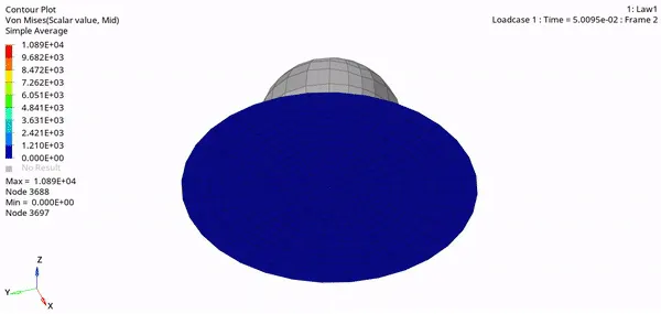
Von-mises stress contour

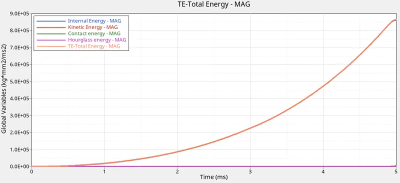
Time vs IE_KE_CE_HE_TE

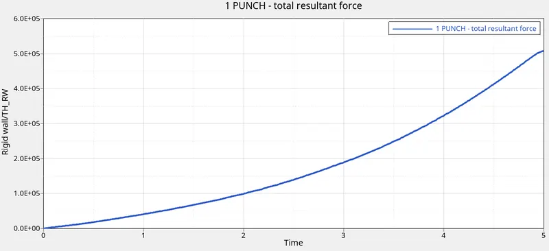
Time vs Resultant force(N) on the rigid sphere

i. In case 5 , we have changed the material model to law 1. In this case the material is assumed to be undergoing an elastic deformation throughout the simulation

ii. The energy plots are similar in shape to case 4 but the values are significantly higher.This is due to a higher amount of deformation in case 5 which has increased the internal energy to a much higher value than in case 4

iii. The resultant forces on the rigid forces on the rigid sphere have also increased exponentially during the simulation. The hourglass energy and contact energy remained zero

CASE 6:In case 6 we have change the material model to law 27. This law combines an isotropic elastoplastic Johson cook material with an orthotropic brittle failure mode

Repeat steps

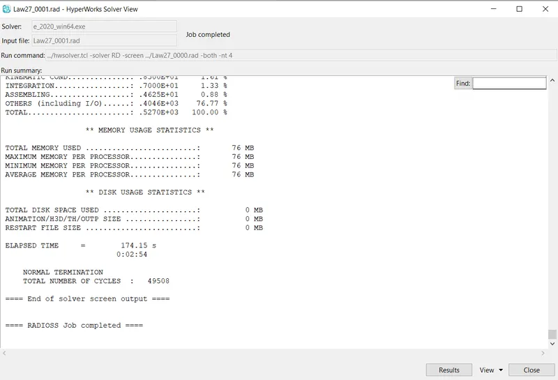
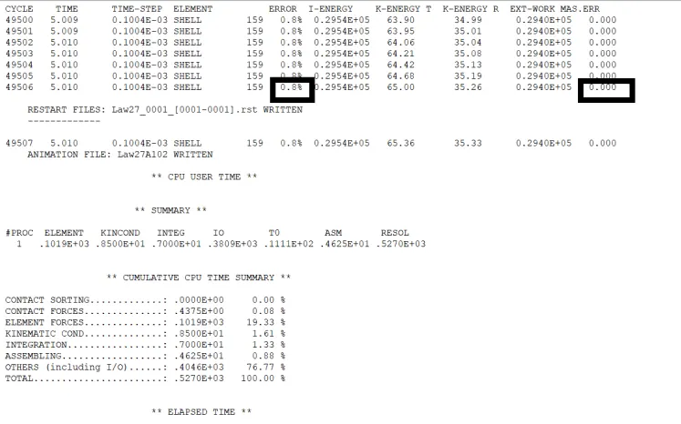
Here the mass and energy errors are acceptable hence we proceed for the simulation part.

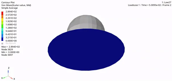
Von-mises stress contour

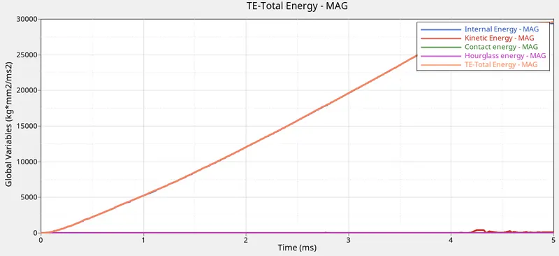
Time vs IE_KE_CE_HE_TE

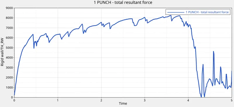
Time vs Resultant force(N) on the rigid sphere

i.In case 6 we have change the material model to law 27. This law combines an isotropic elastoplastic Johson cook material with an orthotropic brittle failure mode. Material damage is accounted for prior to failure.Failure and damage occur only in tension.

ii. Due to brittle nature of the material , the plate can be seen to have cracked from the centre to the edges during the simulation

iii.The energy plots also justify the elasto plastic to brittle transformation of the plate. Also here the IE and TE curves did not flatten out after the breakage of elements

CASE 7: Here we are using law 36 material card.This law models an isotropic elasto-plastic material using user-defined functions for work hardening portions for stress strain curves.

i.Import the model into the solver deck

ii.We then change the properties required for the law 36 card

iii.Next we define a curve for the law 36 card and set fact_ID to the defined curve

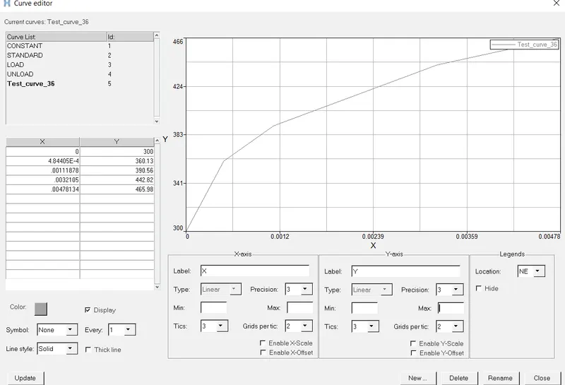
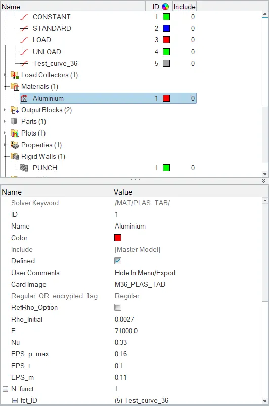
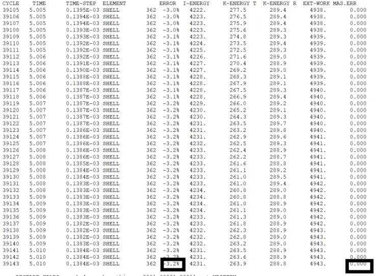
iv. Then we run the analysis [Analysis-->Radioss-->save as-->Radioss]and check the mass and energy results and move ahead to the simulation part

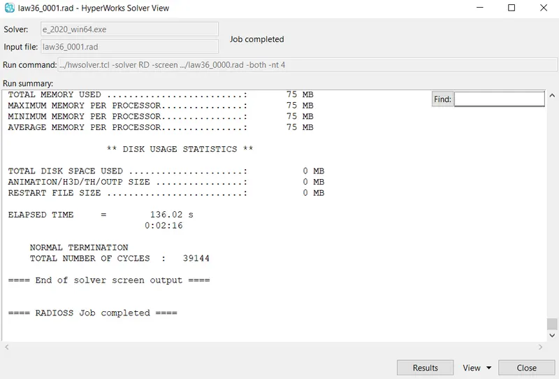
v. Now we post-process our results using hypergraph and hyperview to view the needed contours and plots

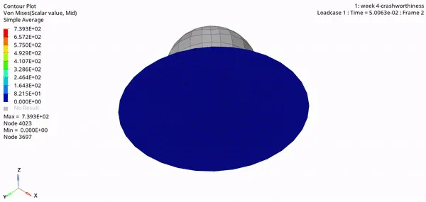
Von-mises stress contour

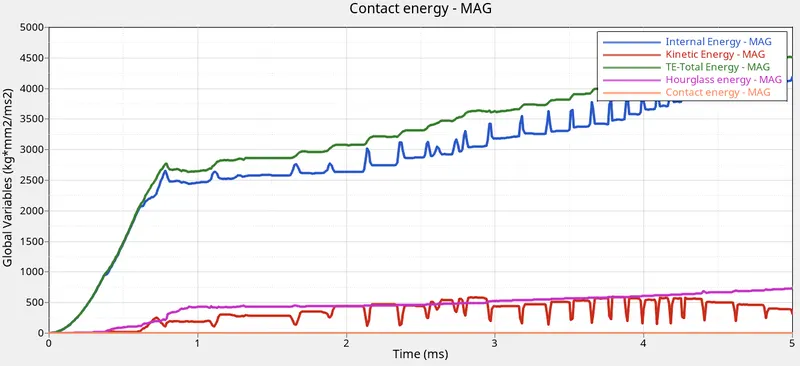
Time vs IE_KE_CE_HE_TE

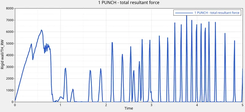
Time vs Resultant force(N) on the rigid sphere

i.In case 7 we have changed the material to law 36(Plas_Tab).This law models an isotropic elastoplastic material using user-defined functions for work hardening portions for stress-strain curves.

ii. The maximum stress is recorded on the first point of contact. As the elements get deleted the plate deforms

iii.The resultant forces on the rigid wall have increased rapidly up to 0.7ms and then we can see a dip which is due to deletion of the center elements due to plastic strain failure. After this dip the forces have fluctuated but have kept on increasing and decreasing

RESULTS:

All 7 simulation were carried out perfectly without any error

Results based on animation

Case_no	Animation	Failure Method
1		Deletion
2		Crack
3		Deletion
4		None
5		None
6		Deletion
7		Deletion

Results based on the plots

Case_no	Plots	Reason
1		The Contact energy and hourglass energy remains zero because of the physical stabilization of hourglass The internal energy of the plate increases linearly due to the absorption of KE from impacting surface Nearly constant values after 4m/s
2		Nearly a linear increase in IE and TE till 4.5m/s When compared to case 1 here KE is much smoother because cracking of elements here is much smoother compared to deletion of big chuck elements HGE and CE remains 0 throughout
3		A linear increase in both T.E & I.E till 4m/s then a dip in I.E & corresponding rise in KE There is a hike in KE graph due to deletion of chuck of elements HGE and CE remains 0 throughout
4		A non linear increase in both IE & TE The Contact energy and hourglass energy remains zero because of physical stabiliation of hourglas
5		The KE gradually increases as the plate stretches to maximum The Contact energy and hourglass energy remains zero because of physical stabilization of hourglass
6		The Contact energy and hourglass energy remains zero because of the physical stabilization of hourglass The internal energy of the plate increases linearly due to the absorption of KE from impacting surface
7		The Contact energy remains zero in this case The internal energy of the plate increases linearly due to the absorption of KE from impacting surface After a certain limit till `0.6ms most of the energy curves fluctuates

CONCLUSION:

• The best case for an on-field scenario totally depends upon the scenario,i.e if elastic material has to be studied then Law 1 is most suitable
• If brittle material has to be studied then law-27 is more suitable
• On other situations like ductile material law 2 with XEFM formulation i.e case 2 is suitable because the crack formation is more related to real-time scenario
• Now with respect to the above case of aluminum case 7 stands most close to real-time scenario as it gives more control and accuracy over the results comparatively