Assignment 3-2D Element Formulation Challenge

# Assignment: 3

Aim: To study the crash Analysis of S-Beam with or without recommended shell formulations in Radioss, and comparing the result with base simulation and improved shell element properties.

Objective:

Various changes and steps need to done in order to achieve the desired outcome

1. Using the crash beam file from the assignment, change the run time to 55ms
2. Change the number of animation steps during simulation to minimum of 25 and maximum of 60
3. Run the base simulation without any modification to element properties
4. At the end of simulation do the energy error and mass error checks and determine whether result should be acceptable or not
5. If acceptable, Plot rigid wall forces, internal energy, Hourglass energy, contact energy, total energy of the simulation
6. Change all the shell element properties to recommended properties, save this file as separate and run the simulation
7. Follow step 5 and 6
8. After that we have to compare the result and need to find the change in result, and if there is change in result then why there is change in the result.

Firstly, we have to understand about the Element Formulation and various parameters which impact the simulation, from this we can get idea about what errors and changes occur in the simulation result and why these error and changes occur

# Introduction to 2D shell Formulation

Element Formulation:

The process of FEA is to discretizing the component an infinite component to finite elements. The discretization process is carried out not just with one particular type of elements. A component is discretize using 1D,2D and 3D elements based on the requirements. Formulation are kind of defining that element behavior and properties. Formulations are the one which give life to the elements, one can easily create the property by clicking right anywhere in the model browser. Once the property is created it must assign to the proper component collector.

1D Element Formulation:

• 1D elements are created when an element is connected between only two nodes
• The cross-sectional area is assumed to be constant throughout the element
• Examples, Truss, Beam, Spring

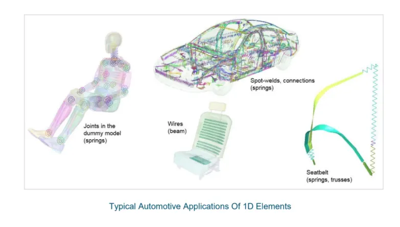
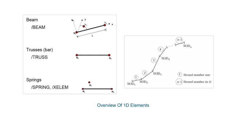
Source: Altair University

PROP/TRUSS

• Similar to beam element but has no bending degree of freedom
• They transmit only axial force and no bending, only translation and no rotation
• Assumed to have constant cross-section
• Compatible with elastic and elastoplastic materials

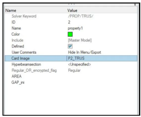
The user must give input to the TRUSS AREA and the Truss activation ID

PROP/BEAM

• They are long and can be oriented anywhere in space
• Has 6 DOF i.e. Both translation and rotation at each node
• A constant cross-section area is assumed
• Node 1 and Node 2 define the element geometry and Node 3 define the cross-sectional orientation

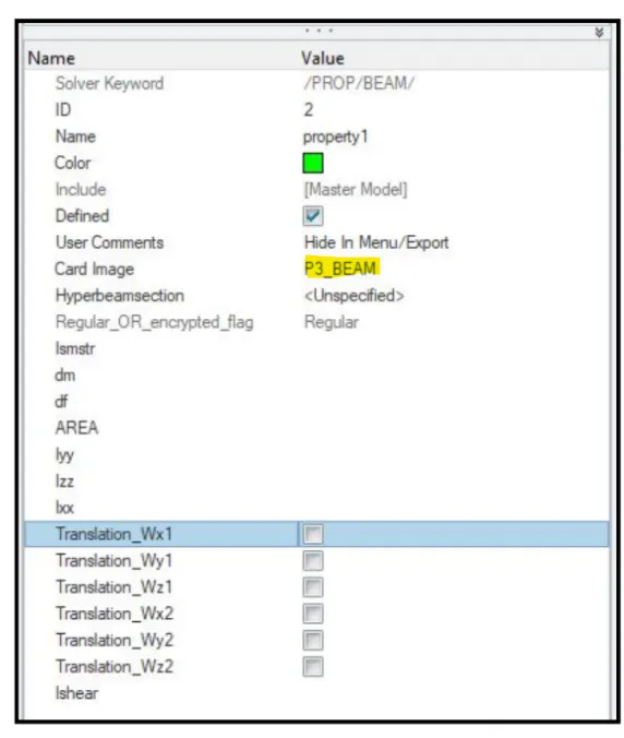
• Here we have Ismstr, which is used to turn on the geometric nonlinearity into consideration
• Area is cross-sectional area
• The inertia of YY, XX, and ZZ can provide only if you have input value or else it is not mandatory
• These check boxes are to define whether the translation and rotation need to be free or constrained, if Box is ticked then DOF is fixed, and if it is unticked then DOF is free

PROP/SPRING

• These elements are commonly used to model connectors in the model
• Linear and variety of non-linear spring are defined for spring through function reference

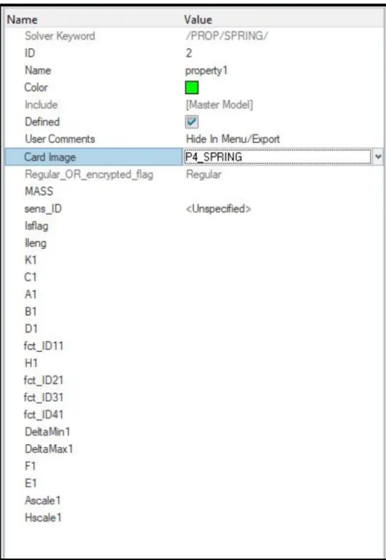
Property card of Spring

• Here we have to define the mass, stiffness K1, Damping C1.
• If spring is non-linear then a variety of non-linear spring option are available under the option H1
• One can define the curve for the spring behavior using the fct_ID11, H1, fct_ID21…. Each function id has its own meaning

2D Element Formulation

• RADIOSS employs shell element as the 2D elements
• Shell elements are combination of Plate elements and membrane elements
• The shell element has 6 DOF, both translation and rotation at each node
• RADIOSS follow mindlin-reissner theory which is nothing but accepting Shear deformation of the shell through the thickness of thin shell and thick shell
• RADIOSS provides both the full integrated and Reduced integrated type of shell element

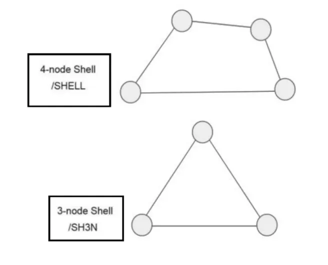
Application of Shell elements

Aerospace, airbag, stamping and automotive full crash, also where the thickness of the model is less than 6mm

Property of shell element

• The mass of shell element is distributed to the nodes
• Shell includes bending and shear deformation while the normal stresses are always zero (Force acting along the thickness of the element)
• Supports large strain with large rotation with bilinear shape function

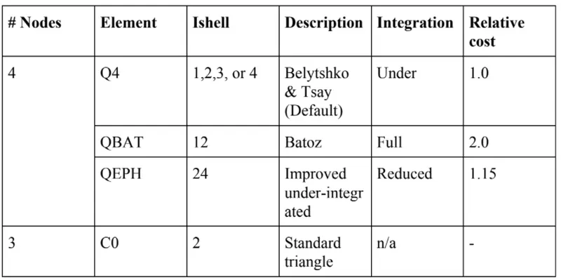
Types of Reduced and full integrated 3 and 4 node shell element formulation

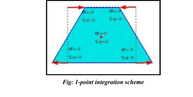
Shell elements: Reduced integration scheme

• Has 1 integration point on the surface at the center
• Widely used in programs with the explicit time integration applied in crashworthiness studies
• Take less time for computation compared to 4 points integration schemes
• Major advantage is that it stabilizes the hour glass mode

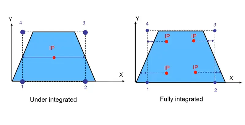
Source: Altair University

Now there is one more important parameter to understand called as Hourglass effect / Hourglass energy

What actually the Hourglass is?

• It is weird mode of deformation that occur in under integrated shell elements when no stresses are produced
• As stresses are not produced, it reduces the accuracy and true response of the structure
• This leads to inaccurate strain and displacement results with unrealistic deformation

When do we say that Hourglass is produced?

• In an under-integrate element, displacements and forces exist for each node of the element
• If the summation of all these forces and displacement provides zero stress and strain on the integration point of the element, then that element fails to calculate the stiffness for the mode of the deformation
• Due to no stiffness calculation, the stiffness happens in a very weird manner
• This is when we call, the element has entered into hourglass

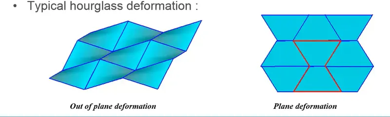
Now we have question in our mind if it leads to give us inaccurate result then how we can control it?

How Hourglass is controlled?

• As mentioned earlier the hourglass occurs only at the under-integrated shell elements. To avoid Hourglass, we go with Full integration scheme or either improved under-integrated scheme
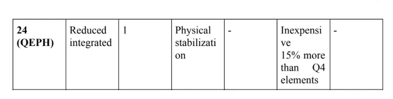
• We saw two type of reduced integration shell elements Q4(I-Shell = 1,2,3,4) and QEPH (I-Shell = 24)
• The control of hourglass also changes on the type of shell element used
• I-Shell = 1,2,3,4(Q4) employs a perturbation method for controlling hourglass
• I-Shell = 24 (QEPH) employs a physical stabilization method for controlling hour-glassing

Perturbation Method:

• In I-Shell 1,2,3,4(Q4) the hourglass motion is detected with motion of the nodes
• If it is detected then opposing force is applied on to the node to stabilize the deformation
• The amount of force inputted is based on the model’s material applied like young’s modulus, yield stress and plastic tangent
• The opposing force produces an artificial energy called Hourglass energy
• One disadvantage is that Q4 elements fail in case of large rotation and elastic loading and unloading cycles

Physical Stabilization:

• In Shell = 24, shell element controls the hourglass from the material level
• Here the hourglass loading stiffness and hourglass yield depends on that material model properties like natural tangent modulus and natural yield respectively
• By this way hourglass is stabilized in QEPH elements
• Advantage over Q4 is that it works perfectly well at all kind of loading and unloading cases

Important parameters in /PROP/SHELL/ [2D Element Formulation]

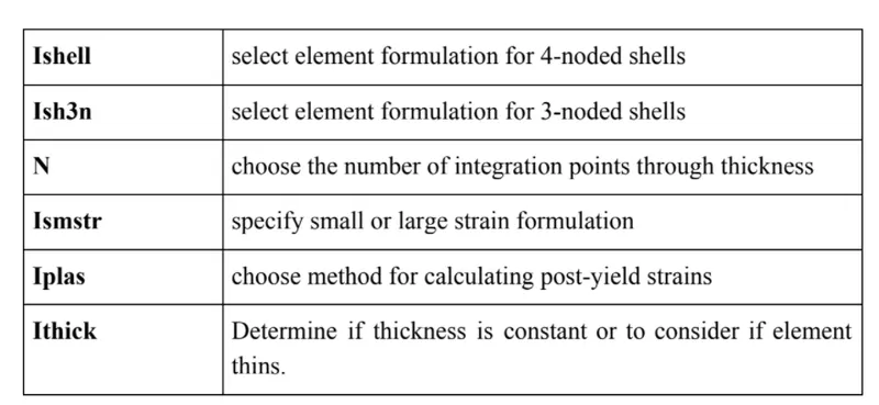
These are all the parameters that we have to lookup during defining of properties for the particular component

PROP/SHELL: I-shell [2D Element Formulation]

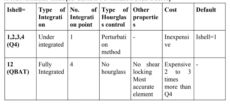
/PROP/SHELL Ish3n = 2

• For tria elements with modification for large rotation
• 1 integration point on the surface
• No Hourglass deformation
• Low cost

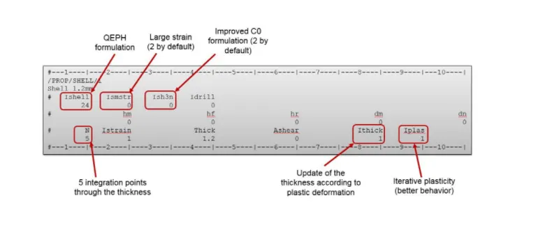
/PROP/SHELL: N- Number of Integration Points

• Up to 10 integration points are accepted through thickness
• 1 integration point through the thickness give membrane behavior
• Recommended N = 5 (i.e. 5 integration point throughout the thickness)

/PROP/SHELL: Ismtr- Strain Formulation

• Ismtr = 1 for small strain from time = o and Ismtr = 2 is a large strain with full geometrical non-linearities
• Small strain occurs when the element undergo small deformation stain is computed on the initial element shape
• Large strain occurs when the element undergoes large deformation, strain is computed
• Recommended: Ismtr = 2

/PROP/SHELL: Iplas- Shell plane stress plasticity flag

• IPlas = 1, iterative projection with three Newtonian interactions, Iplas = 2 radial return
• If the von-misses stress is bigger than yield stress then RADIOSS will:

Update the strain through the thickness

Compute the new thickness of the shell element

Compute the stress using the material law plasticity surface, the strain and the strain rate, the projection of stress on the plastic surface is done with

• Radial return (faster)
• Iterative projection with Newton’s method (more accurate)

Recommended: Iplas = 1

/PROP/SHELL: Ithick-Thickness change

• Ithick = 1 thickness changes is taken into account, Ithick= 2, thickness is constant
• Initial thickness is to compute the strains and to integrate stresses, but thickness variation is still computed for post-processing reasons.
• If Ithick = 1, the change in thickness is not only consider for post processing but also used to compute the strain and stress from true thickness
• For accurate result, iterative plastic projection and thickness variation are employed in the case of breaking, necking etc.

Recommended: Ithick = 1

Source: Altair University

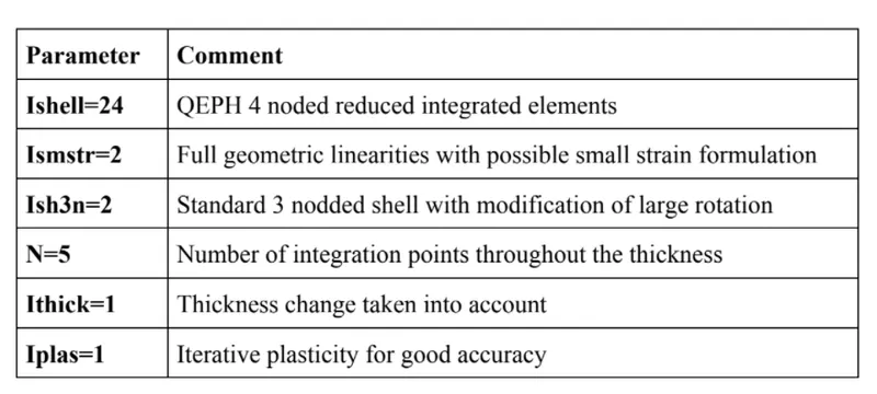
Overall Recommended Parameters for crash application [2D element formulation]

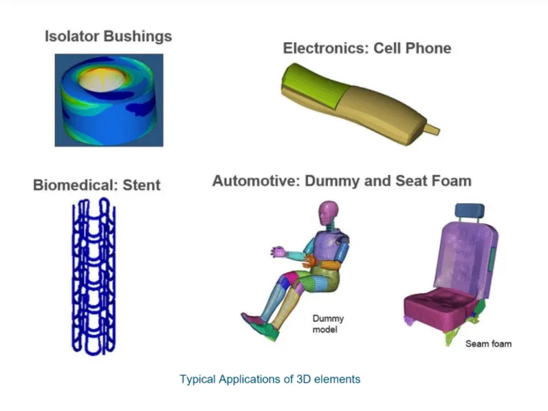
3D Element Formulation

• 3D elements are either tetrahedral or hexahedral element
• Brick or tetra elements may have different number of nodes but support only translational DOF i.e.3D elements have only 3 degrees of freedom.
• 3D elements are used in place where 2D meshing can’t be carried out and if the thickness of the model is more than 6mm
• Both the Hexahedron and Tetrahedron element support linear and quadratic interpolation function
• Linear 3D elements are preferred as they are better in terms of time and memory consumption

Source: Altair University

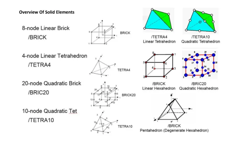
Solid Element Types [2D element formulation solid]

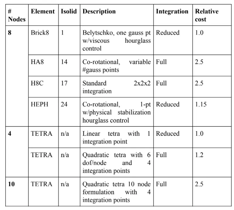
Important Parameter of /PROP/SOLID

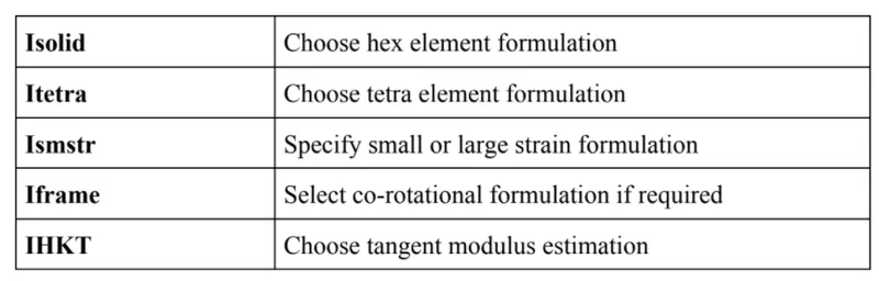
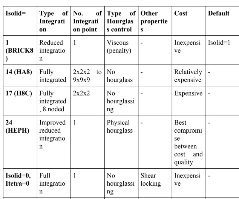
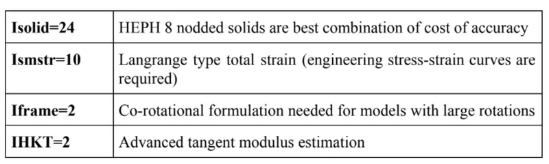
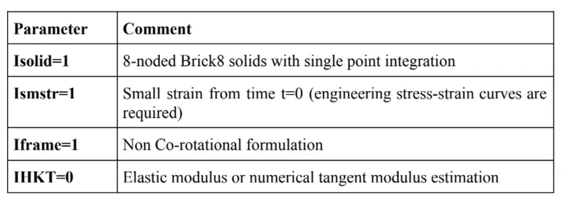
/PROP/SOLID: Ismtr- Solid strain formulation

• Same 2D Formulation is followed for 3D as well
• Follow a large strain with full geometric nonlinearities

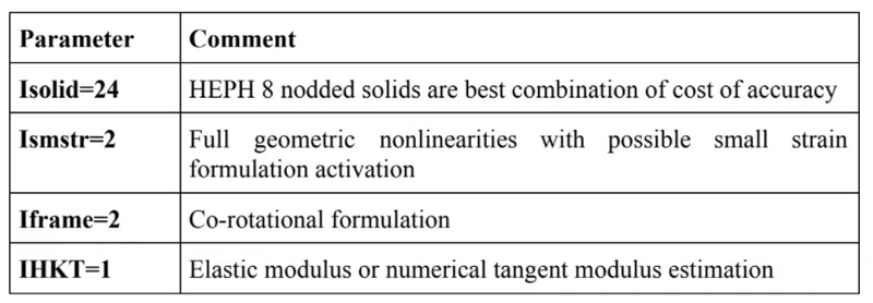
/PROP/SOLID: Iframe- Element coordinate system formulation flag

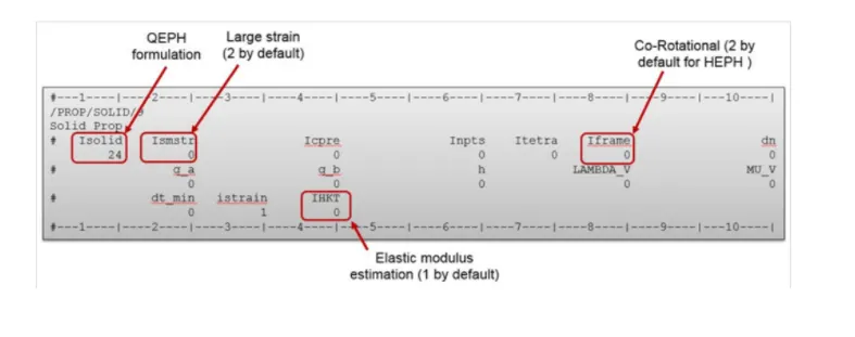
• Iframe = 1 non co-rotational formulation, Iframe = 2 co-rotational formulation needed for models with large rotations (default for HEPH)
• Co-rotational formulation is more accurate if large rotation are involved, at the expense of higher computation cost
• It is recommended in case of elastic or visco-elastic problems with important shear deformation or in case of large rigid body motion

Recommended: Iframe = 2

/PROP/SOLID: IHKT- Hourglass tangent modulus flag

• IHKT = 1 elastic modulus or numerical tangent modulus, IHKT = 2 advanced tangent modulus estimations
• Default for most of cases

Recommended for use IKHT = 2 with HEPH and lagrange type total strain, Ismtr = 10 for foam or rubber materials.

Recommended Solid element Properties for Crash Application

Recommended Solid element properties: For Rubber materials

Recommended Solid Element properties: For Foam Material

S-Beam crash (Without Hourglass Control)

Here we perform small test without any change in the run time and animation file,

Default run time = 60ms (Tstop)

Default animation starting time = 1ms (Animation steps)

After 1ms it start capturing the animation file up to 60ms which is the stop time or termination time of the simulation

Von-misses stresses

Procedure:

• Using the crash beam file from the assignment, change the run time to 55ms

1. Firstly, we import the crash beam file by using import solver deck option
2. The model is in wireframe mode so we need it to change it to shaded mode using shaded element option

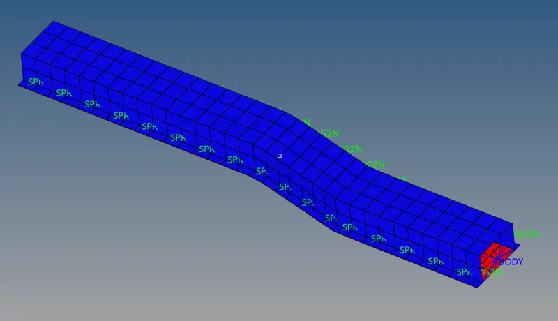
S-Beam

1. We then go to the solver browser option and click on the engine keywords option, here we need to go to ENGINE_RUN to change the termination time to 55ms, instead of 60ms

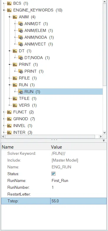
Setting the Termination and stop time to 55ms

• Change the number of animation steps during simulation to minimum of 25 and maximum of 60

1. To change the animation steps during simulations, go to ANIM/DT option in ENGINE_KEYWORDS, here we have to define the time step between minimum and maximum value

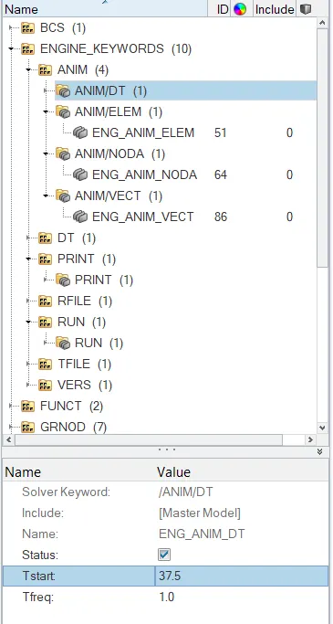
Setting the ANIM/DT parameters

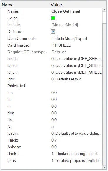
• Run the base simulation without any modification to element properties

Here we don’t need to modify any element property and keep it as default for all parts of model as shown below

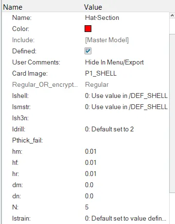
Default properties

• Now next step is to run the simulation with default element property, for that go to Analysis then go to RADIOSS option, we have to define some values.

Options is help us to choose the number of cores you want to use to solve this problem, here we choose 4 number of cores by (-nt 4) after that click on radioss to solve the problem

When, Solving is start, the Solver window is open where you can see the activities that solver perform also if there is any error then it throw you message of warning and error.

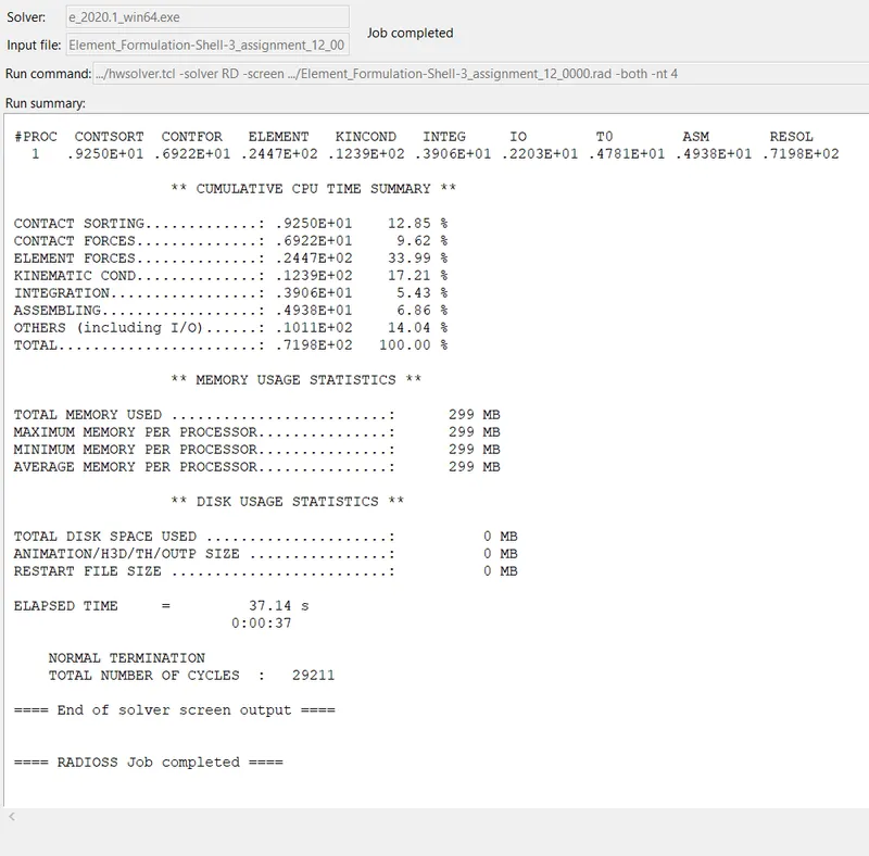
After completion of task radioss will give you message of job completed, here we can also check the weather there is any error present or not

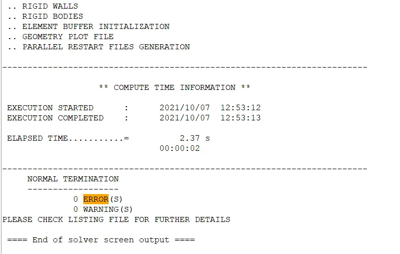
RADIOSS solver will show us 0 ERROR and warning

• At the end of simulation do the energy and mass error checks and determine whether result would acceptable or not

After simulation is complete, go to the folder where the output file has been saved, opened the output file 0001.out file in text editor to check the energy and mass error.

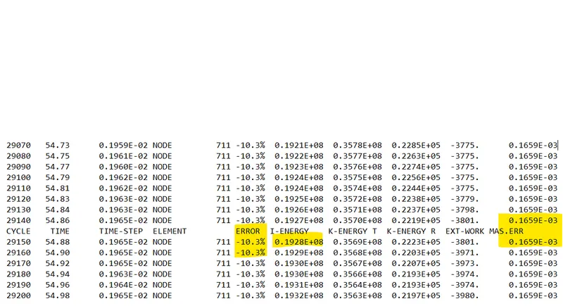
Here we the value of maximum energy error and mass error is -10.3% and 0.1695e^-3

• Basically, the energy error must be between -15 to 5 % is acceptable, if the energy error is below negative then result could be acceptable, here we got -10.3% energy error which is acceptable, closer to 0% error better will be the result

• If result is acceptable plot Rigid-wall forces, internal energy, hourglass energy, contact energy and total energy of the simulation

To plot the results, we have to go to Hyper-view and import the h3d file that solver will give us.

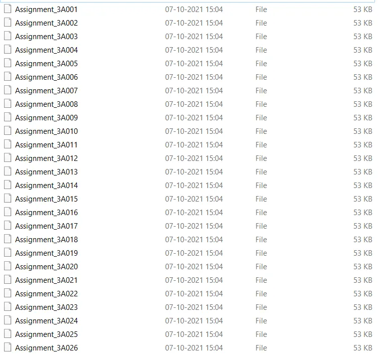
Output Animation files (A01) and Hypergraph files (T01)

After importing the file, we see the beam which is partially deformed, since we have given the animation steps during simulation 30ms, therefore it has start capturing the animation frames after 30ms till 55ms which is our stop time or termination file, the deformed s-beam image is shown below

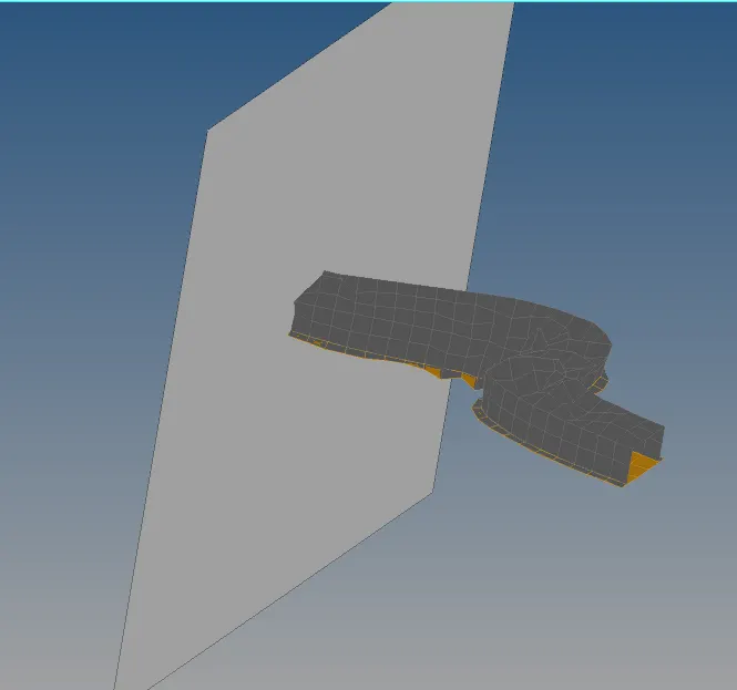
Crushed S-Beam

1. Displacement contour plot

For displacement contour plot we have to go to the contour option present in the hyper-view result tab, under it select the result tab as Displacement and apply it, the max value of displacement we got is 7.611+E+02 at Node 169

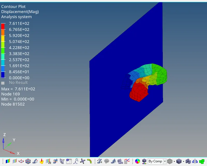
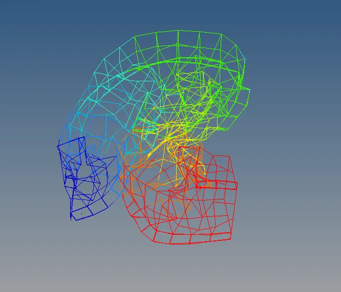
Displacement contour plot

2. Von-Misses Contour Plot

For von-misses contour plot again we have to go to hyper-view result tab, here we have to select the result as von-misses stress, also we have to set the stress averaging methos to simple. The max value of stress we got is 3.5 E+02

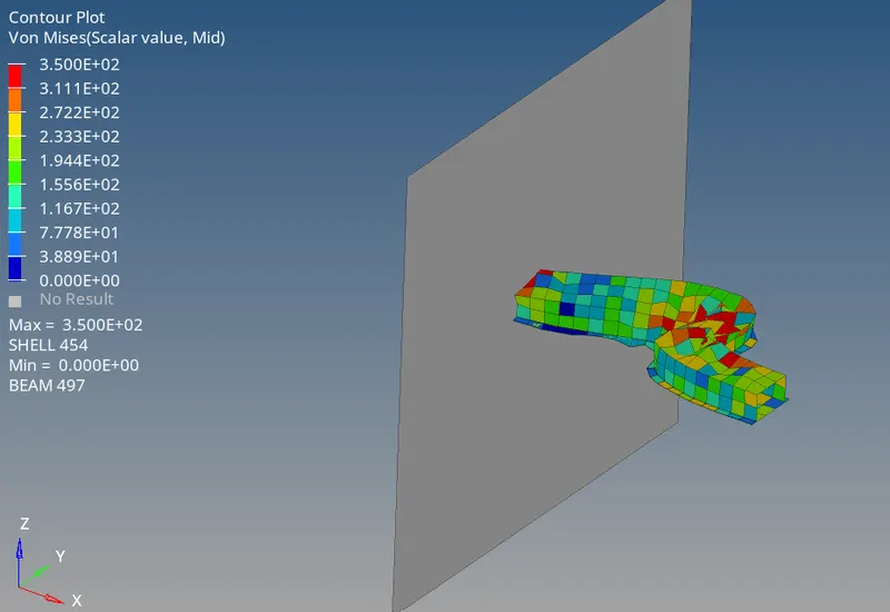
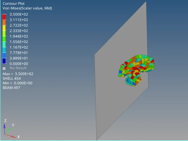
Von-misses contour plot

3. Rigid wall Force 2D plot

For rigid wall force plot, we have to go to hypergraph, here we have to import the T01 file that is output we got, while we solve the problem,

Choose X-type value as time and Y-type as Rigid wall forces, also select the total resultant force that is acting on the wall, and click on apply.

The maximum force we get is 1.14 E+05, The graph is shown in the image below

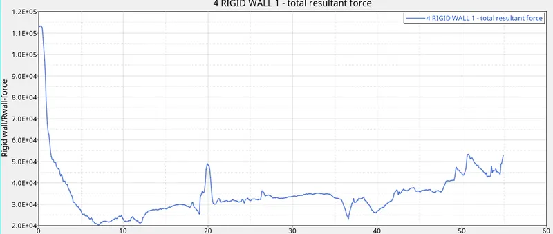
Rigid wall force plot

Here our simulation stops as 55ms because we set the stop time and termination time of simulation to 55ms

Now as you seen here in the graph there is rise and fall in the graph, this is due to because, initially a large force will apply to the wall and after that because the internal deformation inside the beam has started the force that is applied to rigid wall start decreasing, again there is rise in the force because at that situation the bend starts to occur and then with bend the rigid wall force start decreasing, so this up and down is basically but a graphical representation of bend in S-Beam

Rigid wall force → Resultant force → Combination of both normal and tangential Force

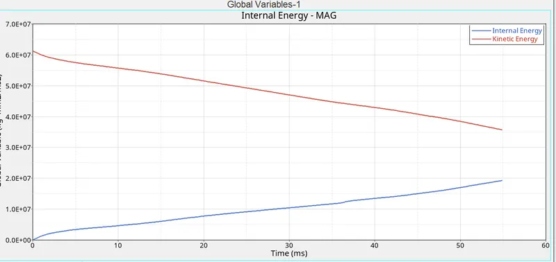
4. Internal energy and kinetic energy 2D plot:

For internal energy and kinetic energy plot we have to select our global variable as internal energy and kinetic energy and plot it against with time, also we have to define the magnitude by selecting Mag option and then click on apply to see the result.

Here as you see the kinetic energy is high at initial level because we have high initial velocity applied to our model which crush them into the rigid wall and with time Kinetic energy start decreasing, also internal energy starts at 0 because there is no deformation take place initially, and with time is start increasing linearly because deformation occur in linear manner, if we run the simulation for more time by increasing the termination time, then you can observe that kinetic energy decreasing and it reaches to 0, also the internal energy reaches to the value where kinetic energy is high at initial level, due to energy losses it can’t reaches to the maximum value.

5. Internal energy, Kinetic energy and total energy

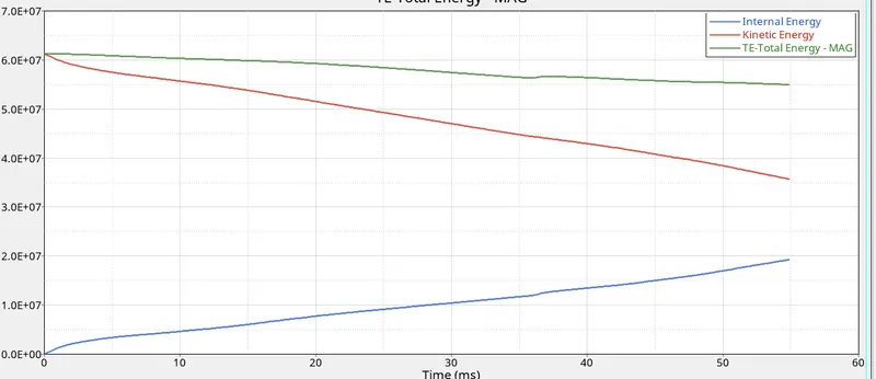
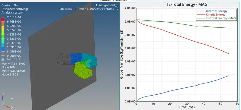
As we see here the internal energy was zero at the initial level and then start increasing as the strain in bream start increasing, so change in the displacement of elements directly effect the internal energy of the beam, so we can say that internal energy is equal to work-done which is again equal to force times displacement. Also, the Total Energy is remains constant, but slightly decreasing with energy losses and due to some energy error.

6. Hourglass energy vs Internal energy

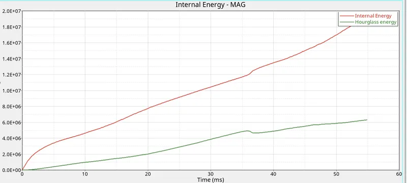
• Comparing Hourglass energy with respect to internal energy or total energy of the system is the best way to identify the hourglass effect in the simulation
• It is recommended that Hour glass energy should not exceed the 5% of Internal energy
• Sometime by manual inspection also we can diagnose the Hourglass energy in the simulation

Here we seen that Hourglass energy is more than 5% of the internal energy, it means that Hourglass energy are involved in our simulation, also by visual inspection it is clearly indicating that hourglass energy is present there, which leads to excessive deformation in the simulation and shows us unrealistic results. So as Hourglass energy increase our result is start deviating from the original result.

7. Contact Energy

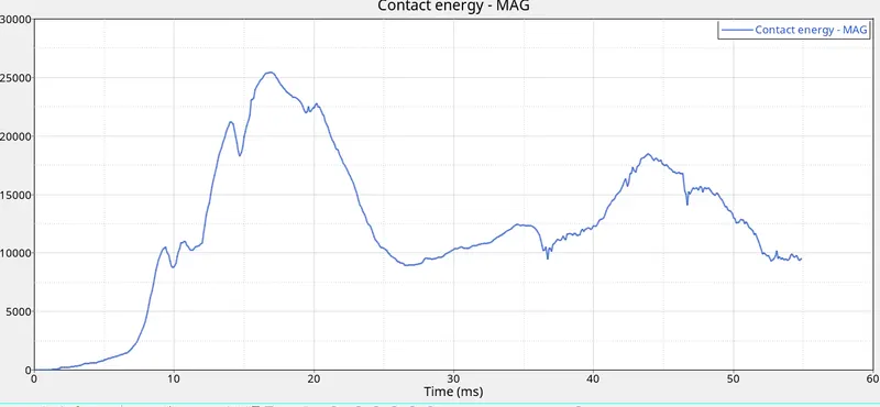
• Change all the shell element property to the recommended property, save the file as separate and run the simulation

Now we have to change the Property of the shell elements, for that we have to go to property section and doing changes in the properties

Recommended Shell element property for crash analysis

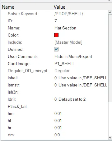
Default property

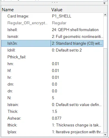
Changes in the properties

• Now after changes in the properties we can run the simulation in same manner as mentioned above

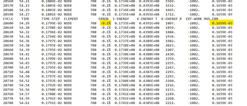
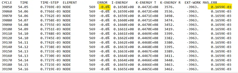
Energy error and Mass error (QEPH, Ishell = 24) Hourglass control

Energy error and Mass error (QBAT Fully integrated scheme)

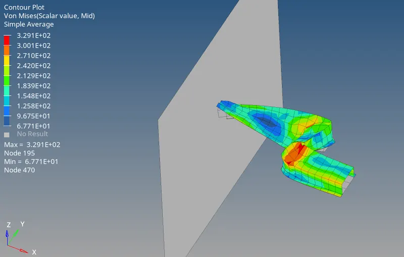
1. Von-Misses contour plot

For von-misses contour plot again we have to go to hyper-view result tab, here we have to select the result as von-misses stress, also we have to set the stress averaging methos to simple. Maximum stress = 3.29E+02 at Node 195

Von-Misses plot

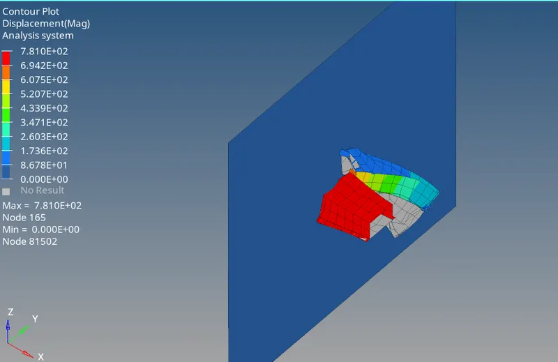
2. Displacement contour plot

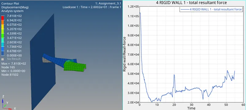
For von-misses contour plot again we have to go to hyper-view result tab, here we have to select the result as von-misses stress, also we have to set the stress averaging methos to simple. The maximum displacement is 7.810E+02 (Node 165)

3. Rigid Wall forces plot

The total resultant force is plotted against time is shown in the image above. The behavior of rigid wall force curve is non-linear, which is due to variation in the force exerted by S-beam on the wall, because it also undergoing bending during simulation that will leads to up and down of the curve.

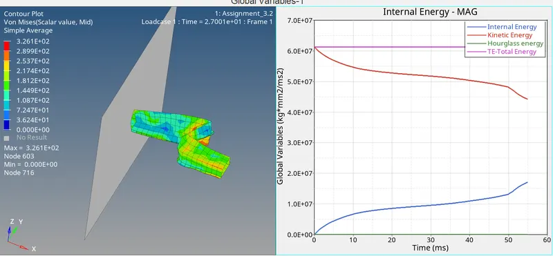
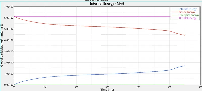
4. Internal Energy, Kinetic energy, Hourglass energy, Total energy plot

Here as you notice that all other things are quite similar, but hourglass energy is now going to 0 and maintain at 0, this means that we apply proper element property that control the Hourglass effect,

5. Hourglass energy

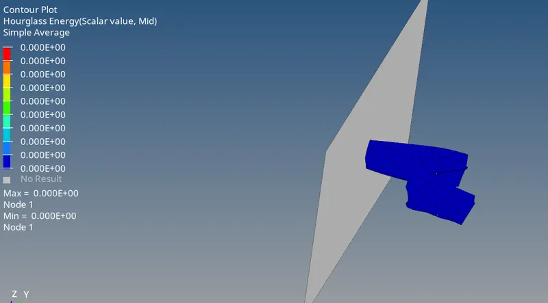
Results with Hourglass control (Hourglass energy is 0)

5. Contact energy

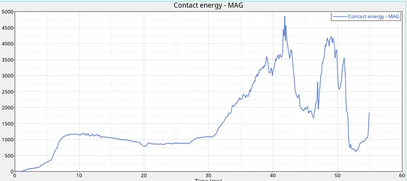
Here the trend of Contact energy is little bit change

The maximum value of contact energy is 4800

• Comparing the Result

1. Contact Energy Plot between default and improved element property (Blue color)

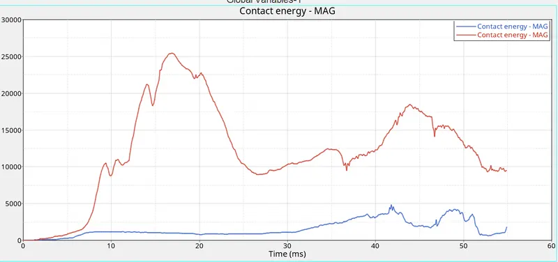
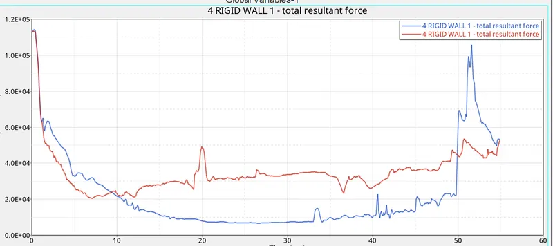
2. Rigid Wall force plot between Default and improved element property (Blue color)

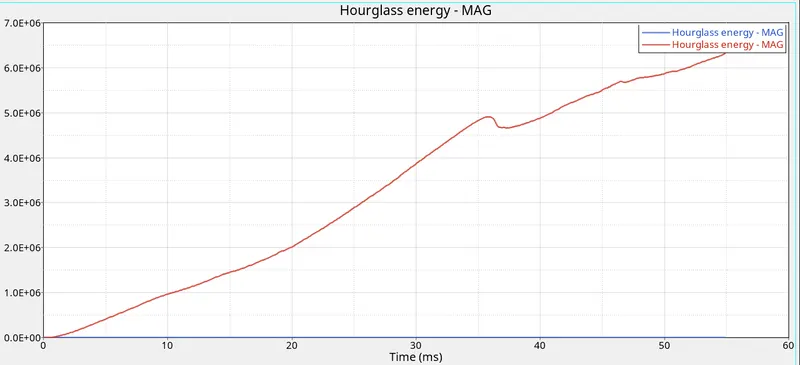
3. Hourglass energy between Default and Improved element property

Hourglass energy is Zero for case where we improve the element property as per recommendation for crash analysis. From this we can say that we can very well control the Hourglass effect if we set property properly as per recommendations.

Conclusion:

1. Total energy remains constant rather than decreasing because energy error reduces to 0.1 % for QEPH and if we are using Qbat then energy error becomes 0%, but Qbat element formulation will uses the full integration scheme, that’s why we got accurate result, but it takes more time to solve, so that’s why we choosing QEPH as our element formulation because it is a best combination of cost and accuracy.

2. Hourglass energy which was increasing changed to zero, so by using proper element properties we can very well control the hourglass effect.

3. Rigid wall force value decreased to lower value than that of default value

From contour plot we can see that there is slight increase in the maximum displacement of the element with recommended property

Hourglass Energy:

What actually the Hourglass is?

• It is weird mode of deformation that occur in under integrated shell elements when no stresses are produced
• As stresses are not produced, it reduces the accuracy and true response of the structure
• This leads to inaccurate strain and displacement results with unrealistic deformation

When do we say that Hourglass is produced?

• In an under-integrate element, displacements and forces exist for each node of the element
• If the summation of all these forces and displacement provides zero stress and strain on the integration point of the element, then that element fails to calculate the stiffness for the mode of the deformation
• Due to no stiffness calculation, the stiffness happens in a very weird manner
• This is when we call, the element has entered into hourglass

How Hourglass is controlled?

• As mentioned earlier the hourglass occurs only at the under-integrated shell elements. To avoid Hourglass, we go with Full integration scheme or either improved under-integrated scheme
• We saw two type of reduced integration shell elements Q4(I-Shell = 1,2,3,4) and QEPH (I-Shell = 24)
• The control of hourglass also changes on the type of shell element used
• I-Shell = 1,2,3,4(Q4) employs a perturbation method for controlling hourglass
• I-Shell = 24 (QEPH) employs a physical stabilization method for controlling hour-glassing

Perturbation Method:

• In I-Shell 1,2,3,4(Q4) the hourglass motion is detected with motion of the nodes
• If it is detected then opposing force is applied on to the node to stabilize the deformation
• The amount of force inputted is based on the model’s material applied like young’s modulus, yield stress and plastic tangent
• The opposing force produces an artificial energy called Hourglass energy
• One disadvantage is that Q4 elements fail in case of large rotation and elastic loading and unloading cycles

Physical Stabilization:

• In Shell = 24, shell element controls the hourglass from the material level
• Here the hourglass loading stiffness and hourglass yield depends on that material model properties like natural tangent modulus and natural yield respectively
• By this way hourglass is stabilized in QEPH elements
• Advantage over Q4 is that it works perfectly well at all kind of loading and unloading cases

General recommendations to check Hourglass energy

• Comparing Hourglass energy with respect to internal energy or total energy of the system is the best way to identify the hourglass effect in the simulation
• It is recommended that Hour glass energy should not exceed the 5% of Internal energy
• Sometime by manual inspection also we can diagnose the Hourglass energy in the simulation

So as Hourglass energy increase our result is start deviating from the original result.

Learning Outcomes:

• Able to understand about the 1D, 2D, 3D element formulation
• Able to understand about importance of the properties, and how it effects the results
• Able to understand about the Hourglass energy and its effect
• Able to understand how we can control the Hourglass energy
• Understanding about how to setup the simulations and how to check the errors and how to debug them
• Able to understand about the different files produced during solving the problem/ simulation, and when to use them, files like A01(Animation files), h3d file, T01 files which gives us result in the form of contour and graphical manner