2D Element Formulation in RADIOSS

2D Shell Element Formulation

Aim

The aim of this work is to inspect the difference between simulation of the crash of beam against the rigid wall with and without modification in element properties.

Objective

1. To change the run time to 55 ms.
2. To change the number of animation steps to a minimum of 25 and a maximum of 60.
3. To run the simulation with and without any modification to element properties.
4. To do the energy error and mass error checks of the simulation.
5. To plot rigid wall forces, internal energy, hourglass energy, contact energy, the total energy of the simulations.
6. To compare the results of the two cases.

Introduction

In the FEA method, the components are meshed using various kinds of 1d, 2d and 3d elements. The idea behind meshing the component is to bring the complexity of solving the equations from infinite level to finite level. After meshing the component, the equations are solved at nodal positions. And using Gaussian integration points, the equations are further calculated for results within the elements. To study the significance of such characteristics of FEA is the objective of this work.

To Change the Run Time and Number of Animation Steps

It was required to set the run time to 55 ms. To do that, the solver deck file, Element_Formulation-Shell-3_assignment_0000.rad was imported in Hypermesh, with Radioss profile. In Model → Cards → ENG_RUN → Tstop, the Tstop value was 60 which was changed to 55, as required. The Tstop value is the run time.

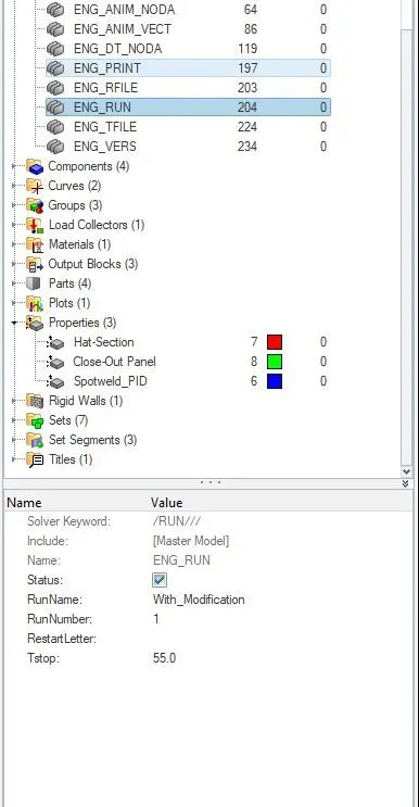
Figure 1: The run time was changed to 55 ms.

Now, the number of animation steps during the simulation was required to a minimum of 25 and a maximum of 60. In this work, the number of animation steps during the simulation was taken as 40. For the value of 40, the Tfreq value is run time per number of animation steps, which is equal to 1.375. Thus, this value was provided to Model → Cards → ENG_ANIM_DT → Tfreq.

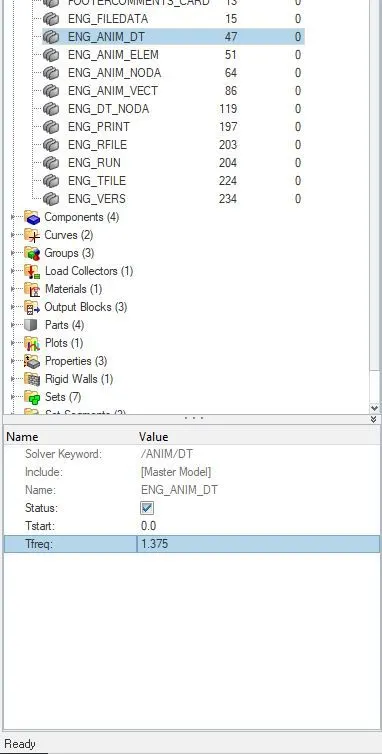
Figure 2: Tfreq was set as 1.375, the value corresponding to the 40 number of animation steps during simulation.

Simulation without Modification in Element Properties

The first simulation had to run with previously set elemental properties. Using Analysis → Radioss, the simulation ran. In the output file, it was observed that the final time was 55, as provided, and the total number of animation files generated was 40, as shown below.

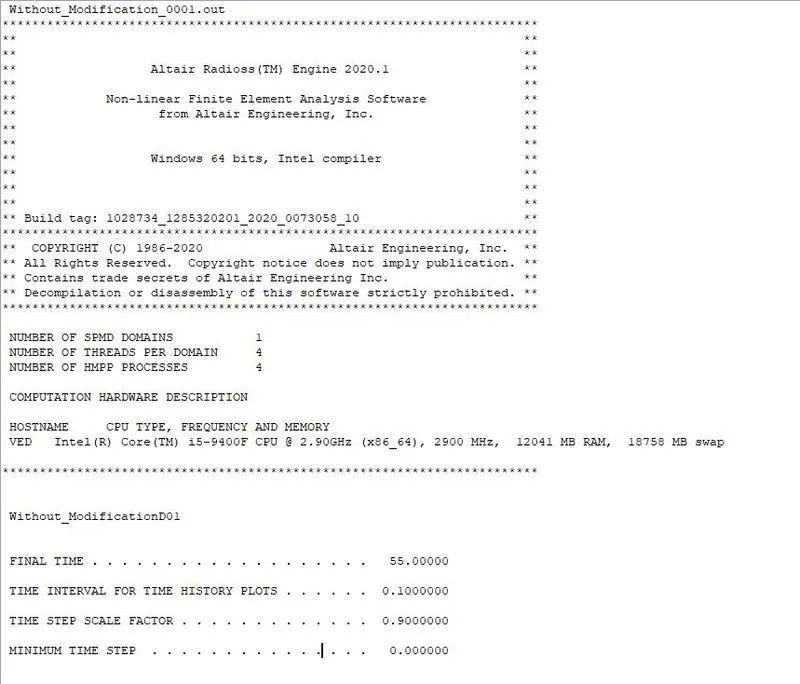
Figure 3: Final time is equal to 55, as provided for the simulation.

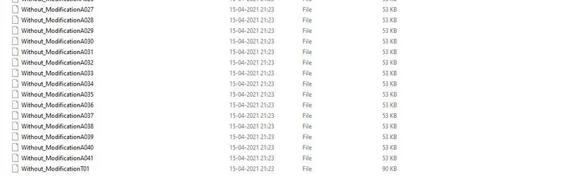
Figure 4: Total number of animation files generated is 40.

In the output file itself, the simulation was observed for energy and mass error. The energy error started with 0.0% and ended with -10.3%, which is acceptable. The acceptable range of energy error is from -15% to +5%. The mass error was constant throughout the simulation with the value of 0.1659e-3, which is also within the acceptable limit. The acceptable limit for mass error is up to 2.

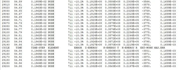
Figure 5: Maximum energy error can be seen as -10.3% and mass error as 0.1659e-03.

After, analyzing the output file, the result was checked for further parameters. When the simulation status has shown that ‘Radioss Job Completed’, it can now be view in Hyperview. So, the accomplished simulation is opened in Hyperview and Von Mises Stresses is obtained using contour, as shown below. From this contour, it is found that the maximum stresses of 349 units are getting generated on the elements which are getting highly compressed, and the minimum stress is on spring elements. Moreover, the mode of deformation of the beam is no seem to be so practical.

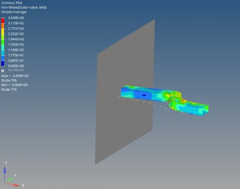
Figure 6: Von Mises stresses the contour of the component without modification in the elemental property.

The simulation is further analyzed using various plots. The first plot was of rigid wall force.

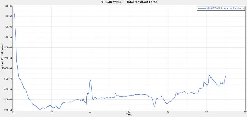
Figure 7: Total resultant force on rigid wall vs. time.

Initially, the force on the rigid wall was maximum, until the force was experienced by the other elements of the beam. Once the other elements, or more specifically the element on the bent of the beam, started experiencing the applied force, the rigid wall force suddenly decreases. When the beam started buckling, the rigid wall force added again.

Next, the internal energy, hourglass energy, contact energy, and total energy of the simulation are plot against time.

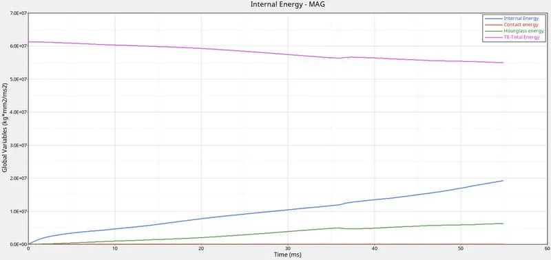
Figure 8: Various plots against time.

In this plot, the internal energy was at zero initially and then started increasing as the strain in the beam started increasing. Change in the displacement of the elements directly affect the internal energy of the beam, as internal energy is equal to workdone which is equal to force times displacement.

The total energy is the sum of kinetic and potential energy. In this simulation, no potential energy is present, thus total energy is directly proportional to kinetic energy. Now because of initial velocity, initially the total energy was at its peak and then started decreasing with a fall in velocity.

Initially, as there was no contact present, between the beam and rigid wall as well as within beam elements, the contact was energy was zero at the start. Once simulation initiated, the contact between elements as well as beam and the rigid wall started increasing, and thus the contact energy started increasing.

Hourglass

The concept of hourglass comes into the picture when any component gets deformed but its strain value does not get recorded. It is also called the zero-energy mode of deformation which occurs in under integrated elements. This brings the error or instability in the result. In the plot, as shown in figure 7, the hourglass energy was zero initially. It started increasing as soon as the hourglass gets developed. The hourglass energy is the artificial energy, that the solver develops in order to counter the error that is getting generated due to the hourglass.

There are three methods to counter/reduce this hourglass effect.

1. Viscous Method/Perturbation Method

2. Physical Stabilization

3. Using fully integrated elements

4. Refining the mesh

In the viscous method, when hourglass deformation occurs, the opposing force is applied to the node in the opposite direction to counter this phenomenon which stabilizes the deformation. This generates artificial energy called hourglass energy. Q4 (under- integrated) or I_shell = 1, 2, 3, and 4 use this method.

In the physical stabilization method, the stiffness is added at the material level, and therefore less amount of hourglass energy is needed. QEPH (improved under-integrated) elements use this method.

Fully integrated elements do not experience the hourglass effect because they have 4 integration points near their 4 nodes.

Simulation with Modification in Element Properties

In the next case, the elemental properties are changed as below. Selecting the right type of elemental property helps in improved quality, and accuracy. Also, it helps the simulation to be performed in economic conditions.

Ishell = 24	QEPH 4 nodes shell is the best combination of cost and accuracy.
Ismstr = 2	Full geometric nonlinearities (default) with possible small strain formulation activation in RADIOSS Engine.
Ish3n = 2	Standard 3 noded shell (C0) with modification for large rotation (default).
N = 5	The number of integration points set to 5 for accuracy in bending.
Ithick = 1	Thickness change is taken into account for accuracy.
Iplas = 1	Iterative plasticity for good accuracy.

The above properties were assigned to the component, as shown below.

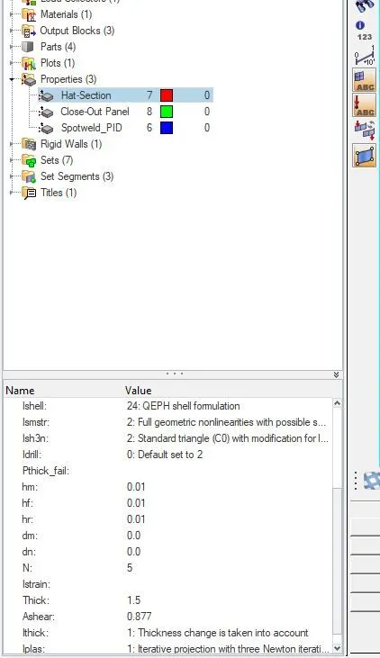
Figure 9: Recommended elemental properties assigned to the component.

Now with these elemental properties, the simulation was performed. The output file showed that the maximum energy error generated is only -0.1%, which is a good improvement.

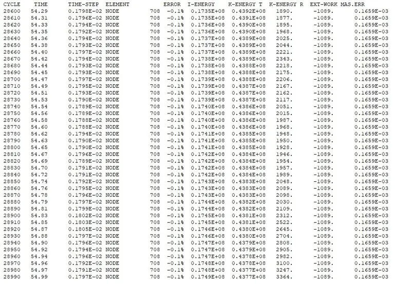
Figure 10: Energy error is reduced to -0.1% which was -10.3% in the previous case.

Figure 11 shows the von mises stress contour with the maximum value of stress of 349 units. Moreover, the mode of deformation has changed after changing the elemental property, and it was quite similar to the real-time scenario.

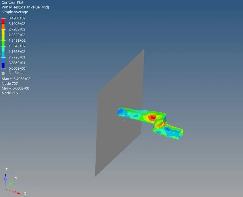
Figure 11: Von Mises stresses contour of the component with modification in the elemental property.

This case is further investigated for the changes in other parameters. The plot for rigid wall force, total energy, internal energy, hourglass energy, and contact energy was generated.

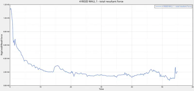
Figure 12: The plot of the total resultant force on rigid wall vs. time for the case with modification in elemental properties.

The plot of rigid wall force shows that after the sudden decrease in the initial force, the force does not fluctuate too much as it was happening in the previous case.

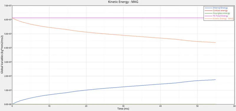
Figure 13: Various plots against time for the case with modification in elemental properties.

In figure 13, the hourglass energy is zero throughout the simulation. It means that the hourglass phenomenon has not generated in the simulation with the modification in the elemental properties. And therefore, the result is much more accurate than the previous case.

Result and Discussion

The case 1 (without modification in elemental properties) when analyzed, the result was in the fitting the in the acceptable limits, as the errors were in acceptable limits. However, the mode of deformation of the component and the increase in the hourglass energy are quite unacceptable issues that have to be taken care of.

With the modification in the elemental properties both of these issues (mode of deformation and increasing hourglass energy) have been resolved. It is because, with the help of QEPH type of shell elements, a physical stabilization happens which helps in reducing the hourglass phenomenon. And therefore, because no hourglass is happening, it means that the strain recording is perfect, thus the mode of deformation is improved.

CONCLUSION

There are various types of elements, and various types of methods to solve the equation within elements. The method is available for the very accurate result, as well as the result close to the accuracy. The selection of solving method depends on the user, that what kind of accuracy he wants, what kind of analysis he’s performing, and how much cost he can bear. The recommended properties for case 2 simulation i.e. with modification in elemental properties, gives very accurate results, and also it is very economical. So, if anyone wants a compromise between cost and accuracy, the properties used in case 2 are a good selection.