Assignment 3-2D Element Formulation Challenge

2D Element Formulation Challenge

Objective:

To perform case 1 & case 2 then Compare both

CASE 1: Run the simulation with the default property with changing the run time to 55 ms with the number of animation steps lies between 25 and 60 and Identify the energy error and mass error, acceptance level.

CASE 2: Run the simulation with the given property with changing the run time to 55 ms with the number of animation steps lies between 25 and 60 and Identify the energy error and mass error, acceptance level.

Given properties:

Parameters		Comment
Ishell =24		QEPH 4 nodes shells are best combination of cost and accuracy.
Ismstr=2		Full geometric nonlinearities (default)with possible small strain formulation activation in RADIOSS Engine.
Ish3n=2		Standard 3 noded shell (C0)with modification for large rotation(default)
N=5		Number of integration points set to 5 for accuracy bending.
Ithick=1		Thickness change is taken into account for accuracy.
Iplas=1		Iterative plasticity for good accuracy.

Procedures:

Case 1:

The given rad file is imported to hyperworks which is displayed in Figure 1 and shaded elems view is displayed in Figure 2.

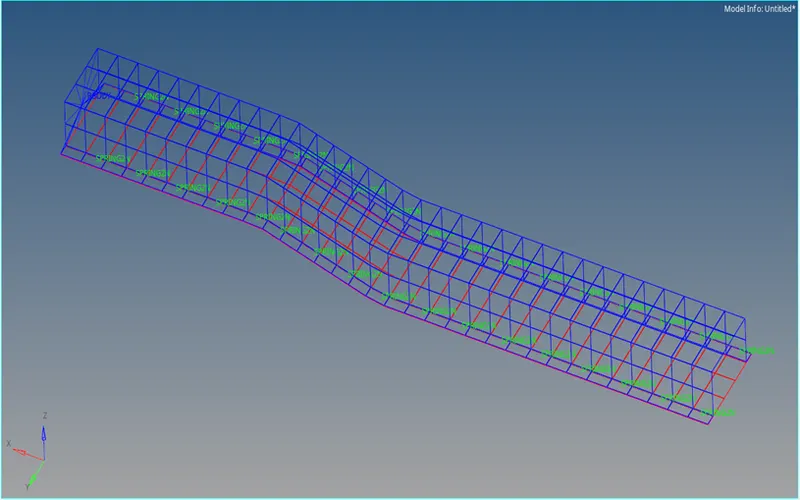
Figure 1: Imported rad file

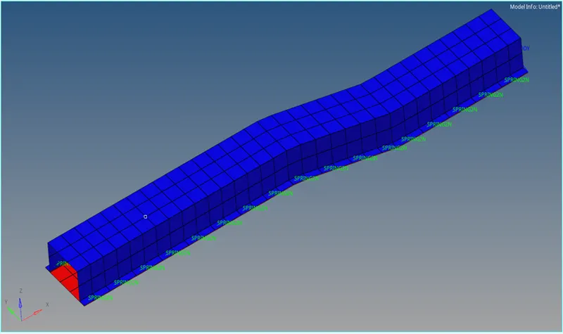
Figure 2: Imported rad file in shaded elems view

Then assign the value of time step in ENG_RUN cars as 55ms as per question as shown in figure 3 and assign the number of animation steps as shown in figure 4.

The T frequency is obtained by assuming 55 number of animation steps which lies between 25 and 60.

Tfrequency= TIME STEP/NUMBER OF ANIMATION STEP = 55/55 = 1

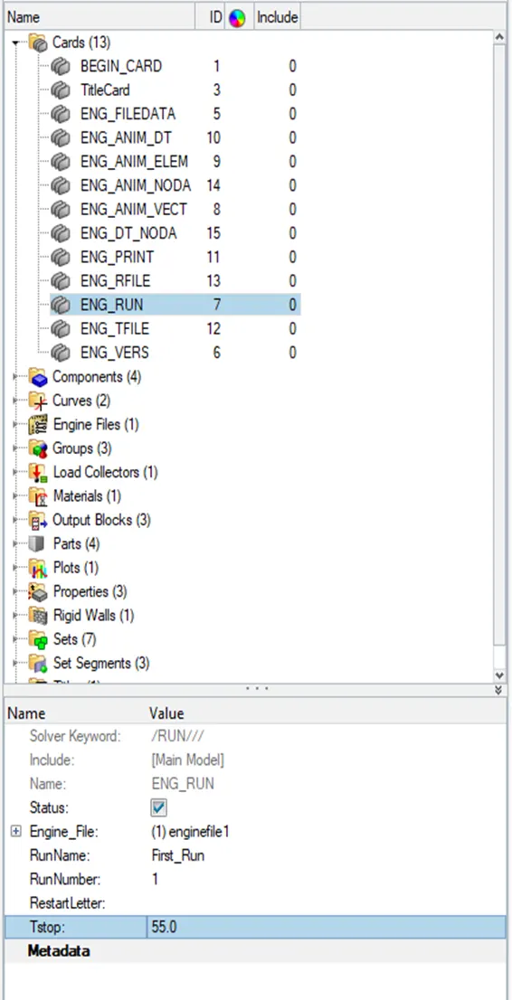
Figure 3: Assigning the value of time step

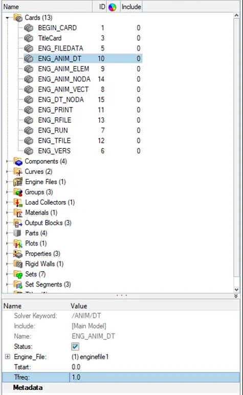
Figure 4: Assigning the number of animation steps

Assign the property card in default shown in figure 5

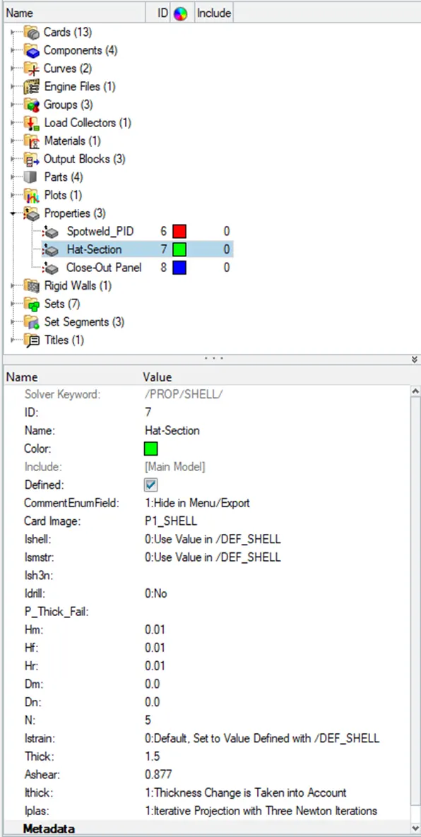
Figure 5: Assigning the property card

To run simulation >> ANALYSIS+RADIOSS as shown in figure 6.

In that panel assign options as -nt 4 as shown in figure 7.

Figure 6: RADIOSS analysis panel

Figure 7: Options panel

After assigning options click RADIOSS and it will show RADIOSS JOB IS COMPLETED in Console solver view tab as displayed in figure 8.

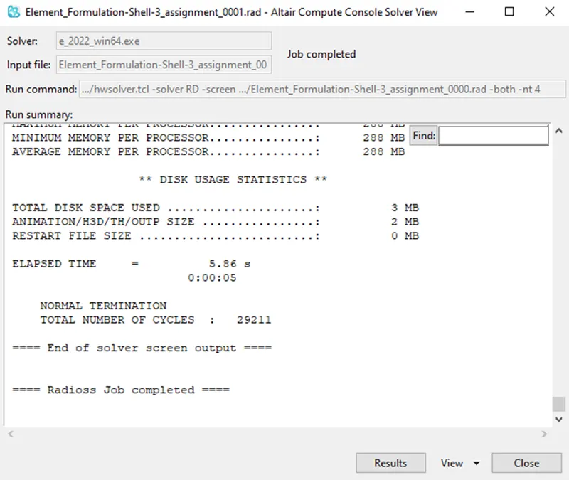
Figure 8: Console solver view tab

Click on RESULT in that tab, it will direct to hyperview where the animation of the simulation is viewed. Animation file are in name of h3d will be in the load area in this panel as shown in figure 9. The animation of the simulation in hyperview is shown in figure 10.

Figure 9: h3d file load area

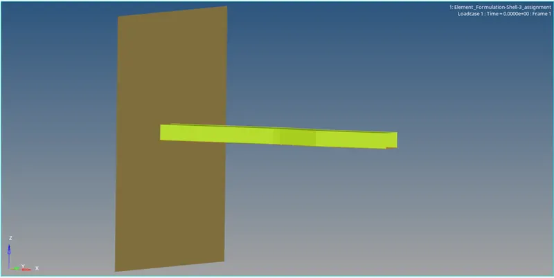
Figure 10: Hyperview

Then switch to contour mode in the panel as shown in figure 11. After switching assign the result type as Von Mises(s) with scalar value as shown in figure 12 and click apply

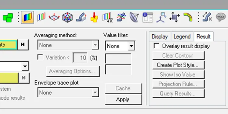
Figure 11: switching of contour mode in Hyperview panel

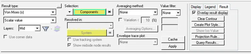
Figure 12: Assigning Von Mises (s)

Result of Von Mises (s) case 1 simulation is shown in figure 13

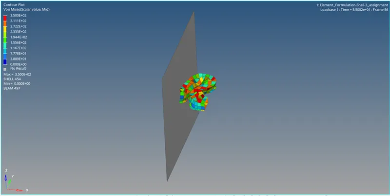
Figure 13: Case 1Von Mises (s) simulation results

Open output of simulation in 0001.out file which is generated after the simulation. We can see the error percentage lies in between the safe tolerance percentage which is -15% TO +5% as shown in figure 14.

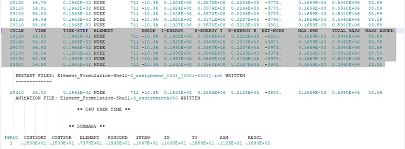
Figure 14: 0001.out file of Case 1

Switch from Hyperview hyper graph to Hyperview 2D then Graphs for plotted for this various energy. For plotting graph, import file T01 which is generated after the Radioss Run. Figure 15 shows the graph of Contact energy, Figure 16 shows the graph of Internal energy, Kinetic energy ,Hourglass energy, & Total energy, Figure 17 shows the graph of total resultant force of Case 1.

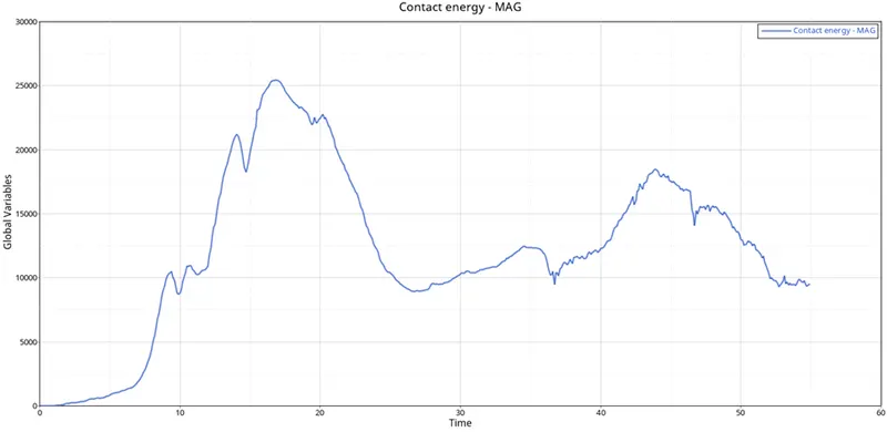
Figure 15: Contact energy-MAG

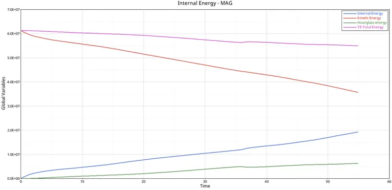
Figure 16: Internal energy-MAG

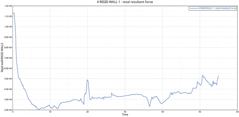
Figure 17: 4 RIGID WALL 1 - total resultant force graph

Case 2

Repeat all the previous steps with add- on step of given property card assigning as shown in Figure 18.

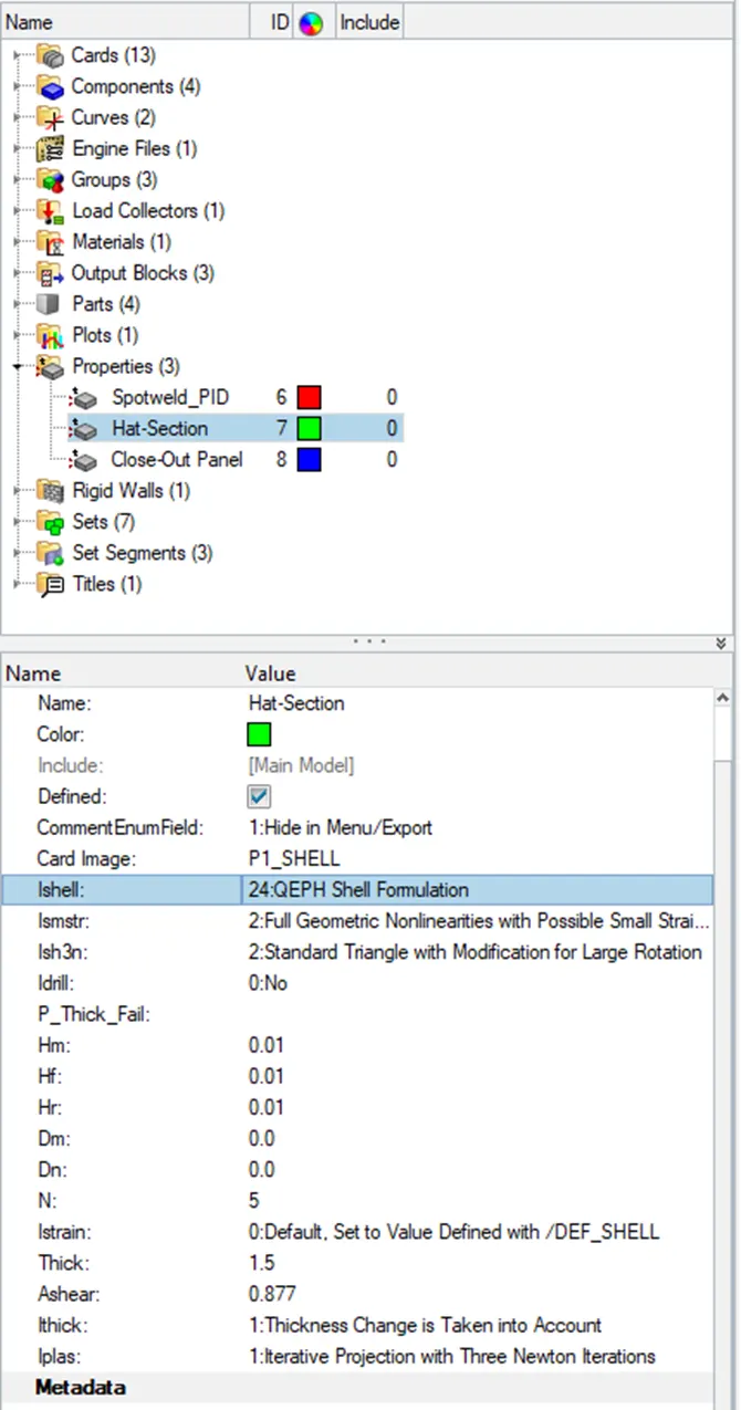
Figure 18: Assigning the property card

Console solver view tab for Case 2 as displayed in figure 19.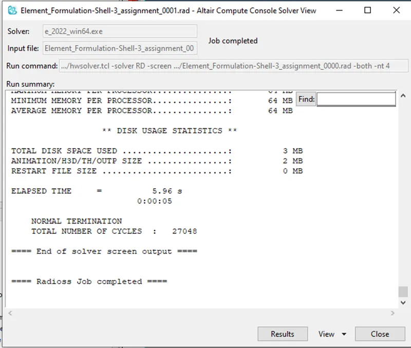

Figure 19: Console solver view tab

Result of Von Mises (s) case 2 simulation is shown in figure 20.

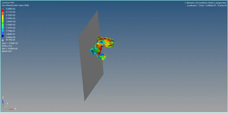
Figure 20: Case 2 Von Mises (s) simulation results

the error percentage lies in between the safe tolerance percentage which is -15% TO +5% as shown in figure 21.

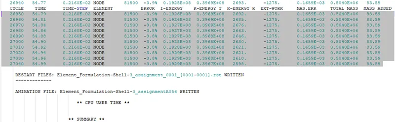
Figure 21: 0001.out file of Case 2

Figure 22 shows the graph of Contact energy, Figure 23 shows the graph of Internal energy, Kinetic energy , Hourglass energy, & Total energy, Figure 24 shows the graph of the total resultant force of Case 2.

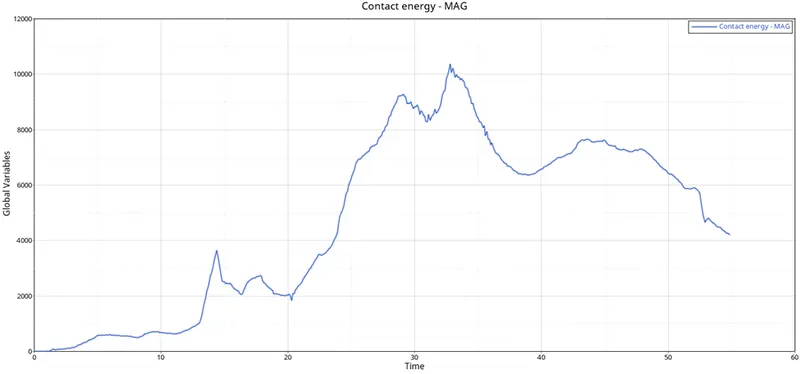
Figure 22: Contact energy-MAG

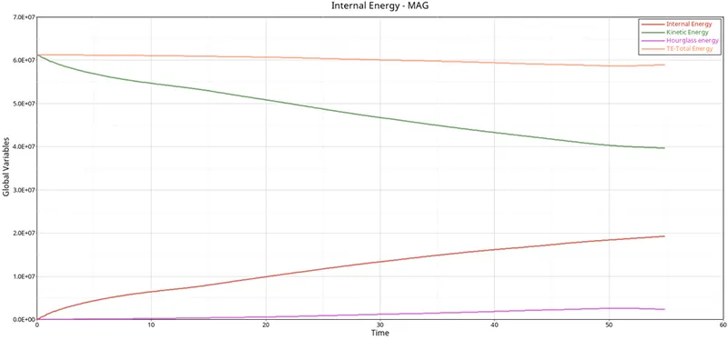
Figure 23: Internal energy-MAG

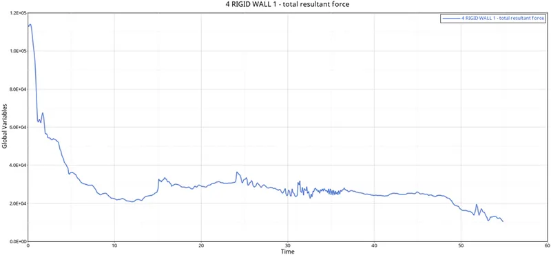
Figure 24: 4 RIGID WALL 1 - total resultant force graph

CASE 1 & CASE 2 COMPARISON

	CASE 1	CASE 2
Contact energy	The peak of contact energy attains between 10 to 20 time steps with global variable 1000.	The peak of contact energy attains between 30 to 40 time steps with global variable 1000.
Internal energy	Internal energy, Rises from the initial point from origin and reaches steadily to 20E+07 with a time step between 50 to 60	Internal energy, Rises from the initial point from origin and reaches steadily to 20E+07 with a time step between 50 to 60.
Kinetic energy	Kinetic energy, Drops from the initial point which is above 6.0E+07 and attains steadily to 3.5E+07 with a time step between 50 to 60.	Kinetic energy, Drops from the initial point which is above 6.0E+07 and attains steadily to 4.0E+07 with a time step between 50 to 60.
Hourglass energy	Hourglass energy, Rises from the initial point from origin and reaches steadily in mid of 0.5E+07 to 1E+07 with a time step between 50 to 60.	Hourglass energy, Rises from the initial point from origin and reaches steadily in mid of 0 to 0.5E+07 with a time step between 50 to 60.
Total energy	Total energy, Drops from the initial point which is above 6.0E+07, and attains steadily 5.5E+07 with a time step between 50 to 60.	Total energy, Drops from the initial point which is above 6.0E+07, and attains steadily in mid of 6.0E+07 to 5.5E+07 with time step between 50 to 60.
Total resultant force	Total resultant force, Drops from the initial point which is above 1.1E+05, and attains a down peak between 5 to 10 time steps then rises again to above 5.0E+04 with a time step between 50 to 60.	Total resultant force, Drops from the initial point which is above 1.0E+05, and attains to1.0E+04 with a time step between 50 to 60.

CONCLUSION:

• All the graph plots clearly show the given time step 55 is reflected accurately in the results since all the plots are ended between 50 to 60 time steps.
• From contact energy plot of Case 1 attains peak value sooner than Case 2. Which is an added point in case of fast contact energy attaining.
• From Internal energy plot of Case 1 and Case 2 doesn’t show consider the level of change in values which shows as a stable variable in both cases.
• From Kinetic energy plot of Case 2 shows that the energy drop is below the value of Case 1. Which is an added point in case of loss of Kinetic energy.
• From Hourglass energy plot of Case 2 shows the minimal energy rise compared to Case 1.
• From Total energy plot of Case 2 shows the minimal energy loss compared to Case 1.
• From Total resultant force plot of Case 2 shows the highest force reduction compared to Case 1, since the values get raised after attaining the down peak.

From the above conclusion Case 2 is more reliable than Case 1.