Assignment 3-2D Element Formulation Challenge

Aim-

• To run the simulation for S-beam with and without changing the recomended prameter for the component using Radioss as solver.

Objective-

• Import the crash beam file and change the run time to 55 sec.
• Change the number of animation steps during simulation to a minimum of 25 and maximum of 60.
• Run the base simulation with default element properties.
• To check the energy error and mass error forthe base simulation.
• To polt the graphs and analyze variation for rigid wall force, kinetic energy, internal energy, hourglass energy, contact energy and total energy.
• Then again run the simulation with change in elements parameter according to given in challenge.
• To plot graphs for 2ndd case also and compare with first case.

What is Element Formulation in FEA?

• The finite element method seeks to offer solutions of displacements arising when loads are applied on a structure. It can also determine the forces that results when a displacement loading condition is imposed on the structure. Finite element meshes play an important role in the derivation of the displacements for a structure.
• Element formulation deals with derivations needed to deduce displacements acting on a body when discretized by finite elements. Different formulations apply for different types of elements.
• Derivation of such displacements is dependent on shape functions.

Types of elements-

1D Elements- Spring, beam, trusses

2D Elements- Quads, Trias

3D Elements- Tetra, Penta, Pyramid, Hexa

2D Element formulation-

• In Radioss 2D elements employs as shell elements.
• The shell elements has 6 DOF ( 3-Rotational and 3-Translational) at each node.
• Radioss shell based on Midlin-Reissner Theory that support of shear deformtion in transverse direction through the thiness of thick and thin shell.
• Radioss provide both fully and reduced integerated 4 noded shell elements.

Diffeerence between fully and Reduced Integerated nodes-

s.no Under Integerated nodes Fully Integerated nodes

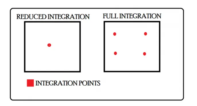
1. It has one integeration points on surface. It has four different integeration points on surface.
2. It save lot of time in simulation calculation . It take lot of time in simulation calculation.
3. It gives less accurate result and less cost. It gives more accurate results and high cost.
4. Hourglass uncontrollable due to underintegerated nodes. Hourglass can be control due to fully integrated nodes.

What is Hourglass?

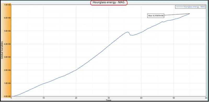
• Hourglass is weird modes of deformation that occur in under integrated elements and no stresses will be produced.This can affect solution accuracy by varying the structure’s true response.This leads to inaccurate stress, strain and deflection results.
• For an under-integrated element, displacements and forces may exist for each node of the element. If sum of all these forces and displacements give null strain and stress on the integration point of the element then that element fails to calculate stiffness for certain mode of deformation.
• At this stage we say element has entered into hourglass. Soon after this as element failed to calculate stiffness the element will behave weirdly.
• Fully integrated solids and shells do not hourglass.

Methods to control hourglass-

1.Perturbation Method Ishell= 1,2,3 or 4 (Q4) [Viscous Method]

• The hourglass deformation is detected with the relative motion(velocity) of the nodes.
• When hourglassing is detected a force is applied on the node to stablize the deformation.
• This force is defined according to the element stiffness (young modulus, yield stress, Plastic tangent).
• This force introduces a artificial energgy termed as hourglass energy.
• Recomended for high stress and high strain rate problems.

2.Perturbation Method Ishell=24 (QEPH) [Stiffness Method]

• Hourgalss yield depend on natural yield.
• Hourglass loading stiffness depends on natural tangent modulus.
• The hourglass treatment is done at material level.
• QEPH is not recomended for orthotropic material.

2D Element Formulation-

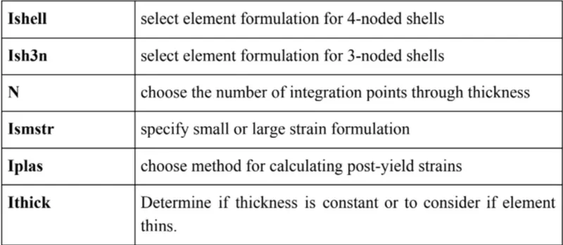
Key parameter for shell elements-

Q4 [Ishell 1,2,3 or 4]-

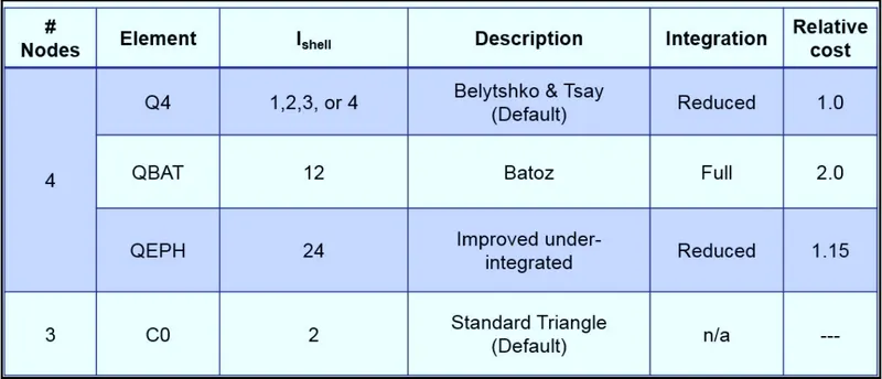
• Q4 is under-integerated 4 node element with 1 integeration point on the surface.
• Default shell formulation is Ishell=1
• Relatively inexpensive.
• Hourglass stablization with perturbation method.

QBAT -

• QBAT is fully integerated 4 noded element.
• 4 Gauss integeration points on the surface.
• No hourglass deformation because its fully integerated.
• Most accurate element formulation but higher CPU cost.

QEPH-

• QEPH is an improved under-integerated 4 node element with 1 integeration point.
• Physical hourglass stablization with stiffness method.
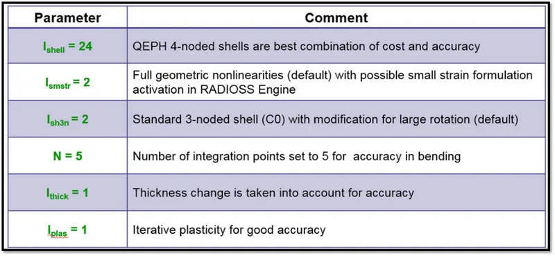
• Its a best compromise between cost and quality ( accuracy of results improved alot).
• It is 15% costlier than Q4.
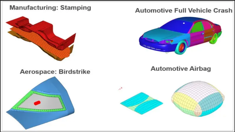
• Best choice for automotives.

CO Element-

• CO is standard triangle (CO) with modification for large rotation.
• 1 integeration point on the surface.
• It has only 3 node ( which needed to form a plane),so there is no chance of deformation from the plane/out of plane.
• So no hourglass deformation.
• Low CPU cost.

N - No of integeration point through thickness-

• In Radioss upto 10 points through the thickness allowed.
• 1 integeration pointthrough the thickness give membrane behaviour.
• N=5 integeration recomended.

Shell stress formulation Ismstr -

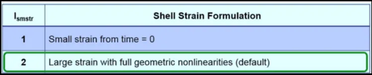
Small strain-

• Usually problems for small deformation.
• Strain computed based on initial element shape.

Large strain-

• For problems with large deformation.
• Strain computed based on current element shape with the derivative of shape function.
• Since in large deformation element size will change drastically so strain calculation should be vary instanteneous.
• Because of size is changed, shape function may stable but the variable in shape function is going to be change like length and gaussian integeration points and due to this whole calculation will change for further step.

Shell stress computation-

• From the deformation and strain rate of previous step RADIOSS Computes the strain to each integeration point.
• From this strain the stresses is computed with elestic stress increment.
• Now with these computed stress value von-misses stress is computed and compared to yield stress of the material.
• If the von-mises stress smaller than yield stress the computed stress is one used in order to compute the internal force of the element.

[Note- If the computed stress is more than yield stress then it will go into plastic region for that we will set Iplas parameter]

Shell plane stress plasticity Iplas-

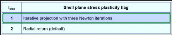
• If von-mises stress is bigger tan yield stress then Iplas will be activated.
• If we will choose 1st option then it will update strain through thickness with new elastic modulus.
• This is why for shell elements needs to be take care of thickness using a thickness value as well as the number of integeration points over the thickness.More the number of integeration point more accurate result we got.
• If we choose 2nd option it will give faster but less accurate result.

[Note- For thickness calculation we should activate Ithick card]

Ithick for thickness -

• Since in some cases if von-mises stress goes beyond yield stress then in that case thickness change will also should be considered.
• Initial thickness is use to compute strains and to integerate stress, but thickness variation is still computed for post processing reason.
• If variable thickness is used, true thickness is not only use for postprocessing but also for strain computation and stresses integeration.

Recomended parameter for shell elements in Crash-

Applications-

Procedure-

Stage-1: Import-

[Note-Import this model using Radioss profile]

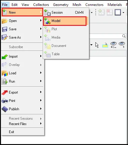
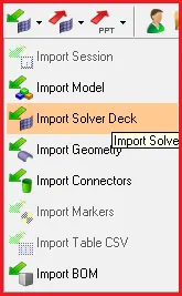
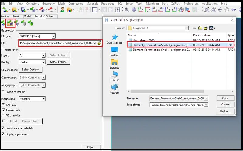
• Here swith the file type Radioss block and then select the file which need to import.
• After importing the file go to model browser and check for cards.

Stage-2:Edit Engine File

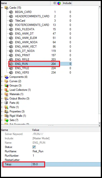
1. Run Time-

• In cards set the Tstop value as 55 which is run time.

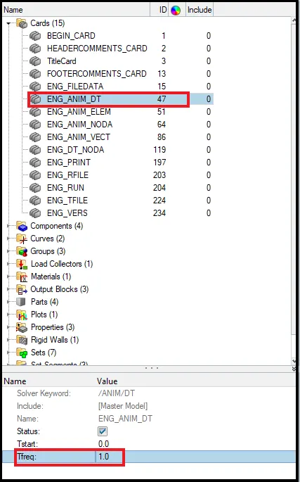
2.ANIM_DT (Frequency)

• And then open ENG_ANIM_DT file and Tfreq value.

Since we will conside animation step as 55,

so Tfreq =Run time/No. of animation step

=55/55

Tfreq = 1

Stage-3: Run the base simulation withouth changing the shell parameter

• will keep the shell parameter as default for 1st case.

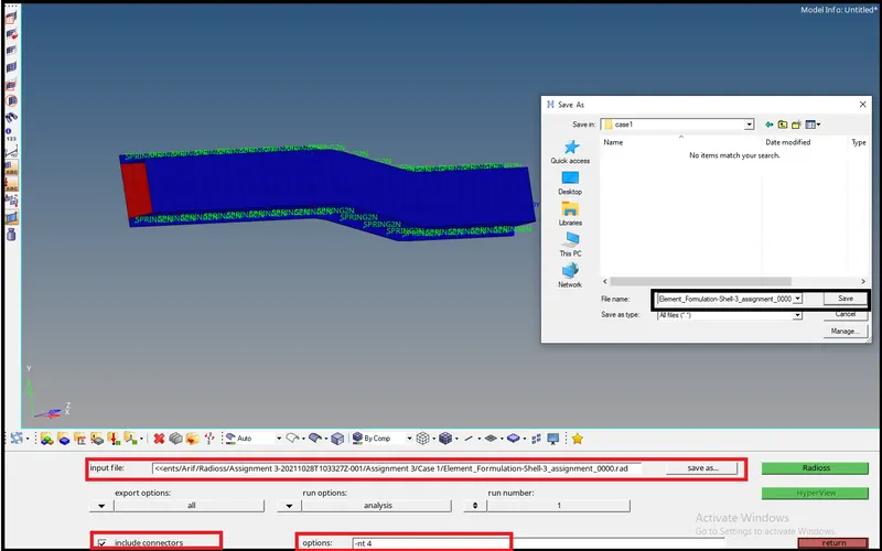
• Now run the simulation in Radioss as shon below.
• Check the include connectors and option as -nt 4.

• Then save this 0000.rad file as desired location named as case -1.

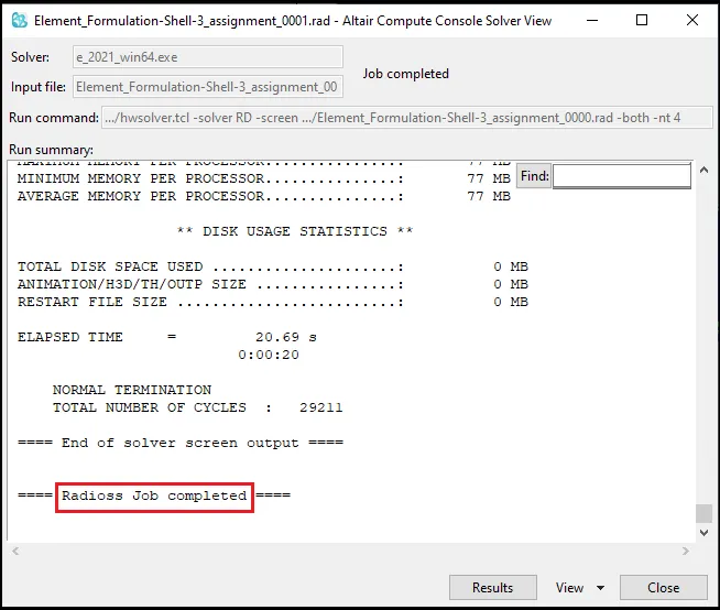
• After that click on Radioss it will start the simulation.
• And wait untill the new window popup and show as Radioss job completed.

• Now open the Engine file (0001.rad) file to varify the Tfreq and Tstop values.
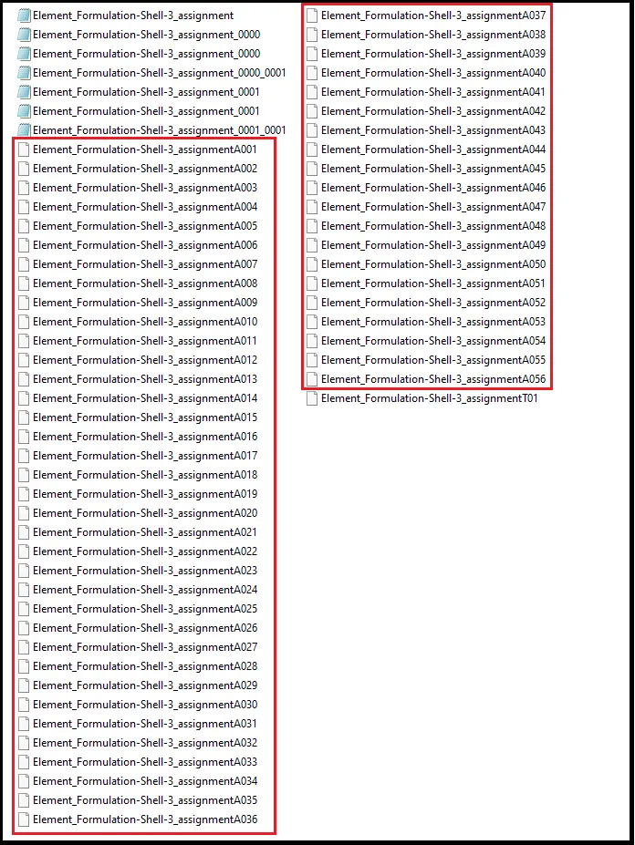
• Now since we assigned the number of animation file as 55 so now then check foe all the file.

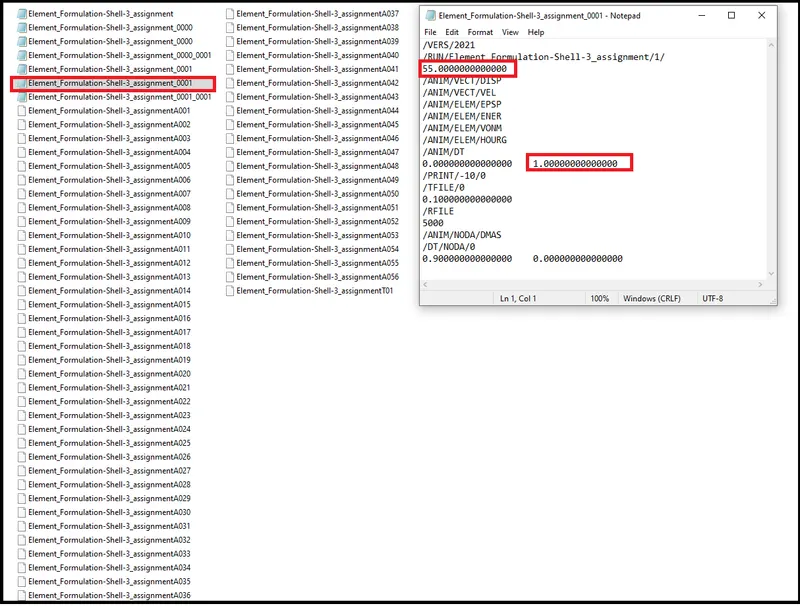
• Here we can see number of animation step as 56 we obtained.

Stage-4: Energy Erros

Check for Energy error and Mass error-

• After analysis two Engine file has generated 0001.rad and 0001.out .
• Now check for energy errors in 0001.out file.

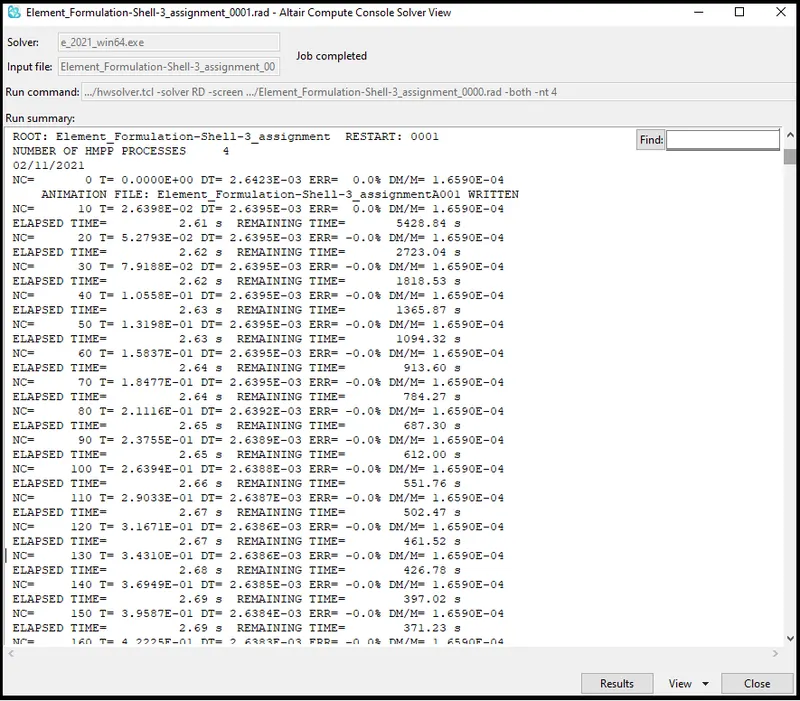
Fig- Engine File[0001.rad]

Types of Energy Errors-

1. Time step
2. Energy Error
3. Mass Error
4. Internal Energy Error
5. Kinetic Energy Error
6. Contact Energy Error

Acceptable range for a. Energy Error is -15% to +5%

b. Mass Error is 0 to 2%

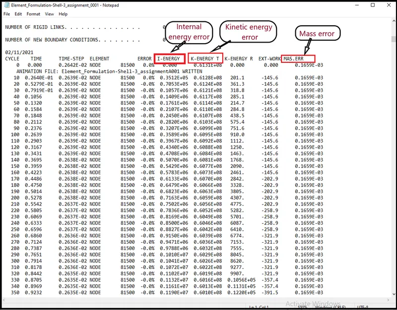
Fig- Engine File[0001.out]

• Now check for maximum error in the list-

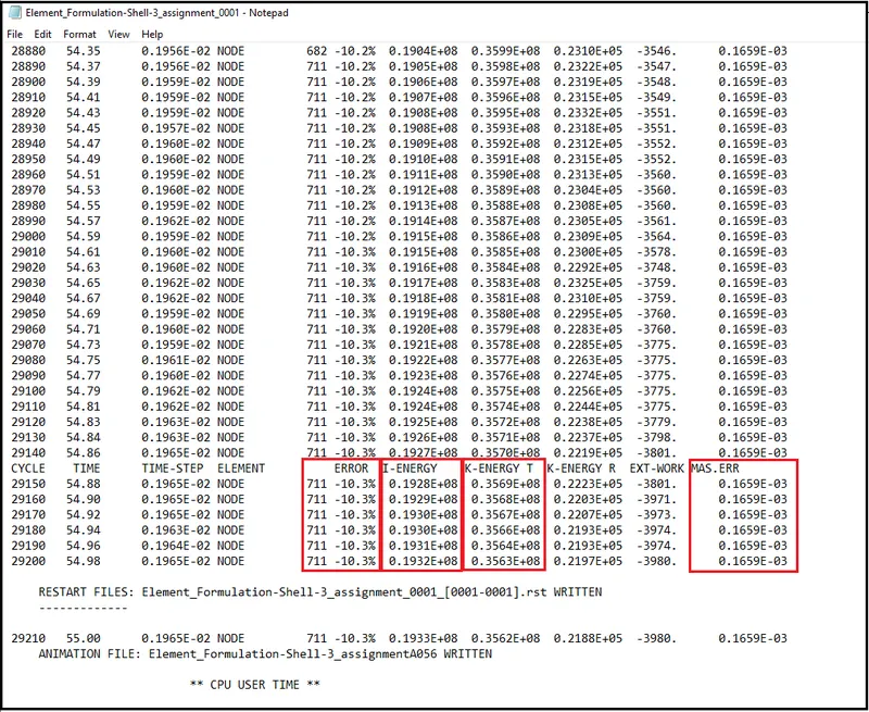
• Maximum energy error= -10.3 Acceptable (Range is -15% to +5%)
• Maximum internal energy error= 0.1932 x 10^8
• Maximum kinetic energy error = 0.3563 x 10^8
• Maximum Mass error = 0.1695 x 10^(-3) Acceptable (Range is 0 to 2%)

Stage-5: Postprocessing

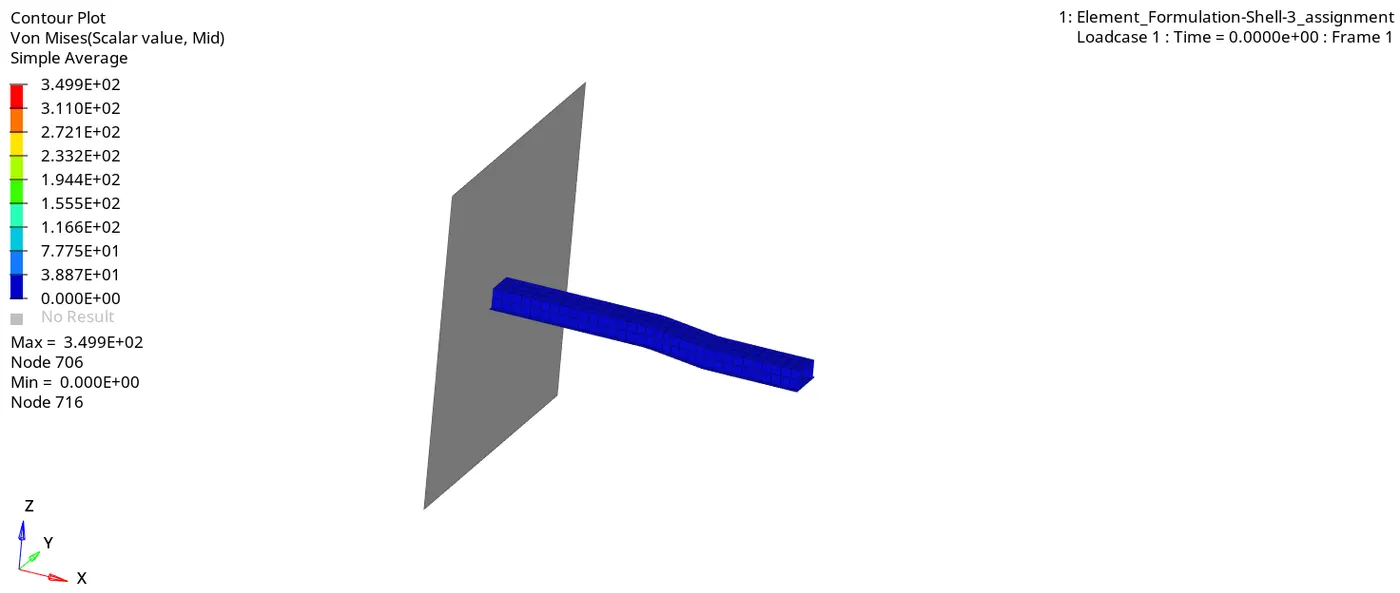
• Review the simulation using Hyperview.
• Plot the graphs using Hypergraph-2D

1.Review the simulation using Hyperview.

Split the screen in two part-

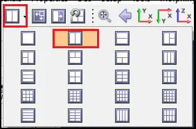
window Splitted-

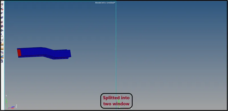
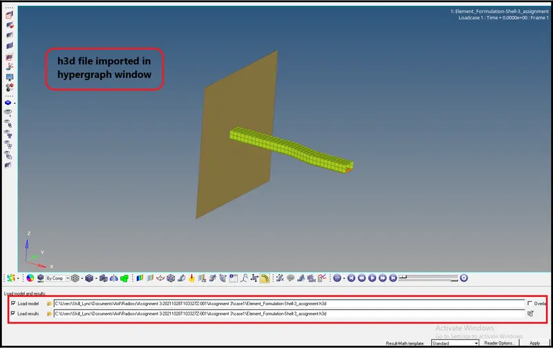
Open Hypergraph-

• In hypergraph window import the h3d file for simulation run.

2. Plot the graphs using Hypergraph-2D

• Now split the window in 3Part and open hypergraph-2D in new window.
• After opening the hypergraph windoe import the T01 file in Hypergraph.

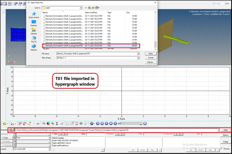
• After importing the T01 file we will start plotting graphs.

Rigid wall force-

Graph-

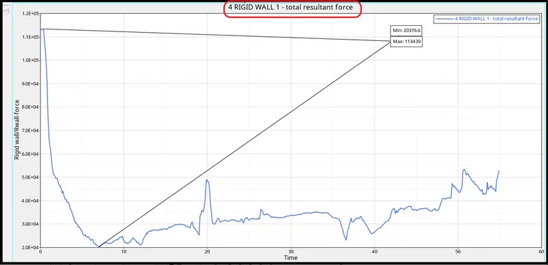
• Rigid wall force is force exterted by rail elements to the rigid wall.
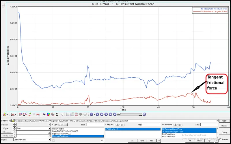
• Initially it was higher but due to internal deformation in rails the apllied force on rigid wall start decreasing.
• Initially force is higher in the gaph because, initial point shown in the grapgh is the moment when rail hits the wall amd at that moment Rigid wall force was high.
• There is significan amount of force which started getting converted into frictional force so we will plot froctional force also.

• Now start ploting graphs for Internal energy, kinetic energy, contact energy, hourglass energy and total energy.

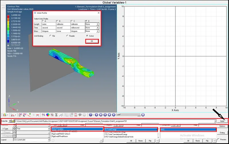
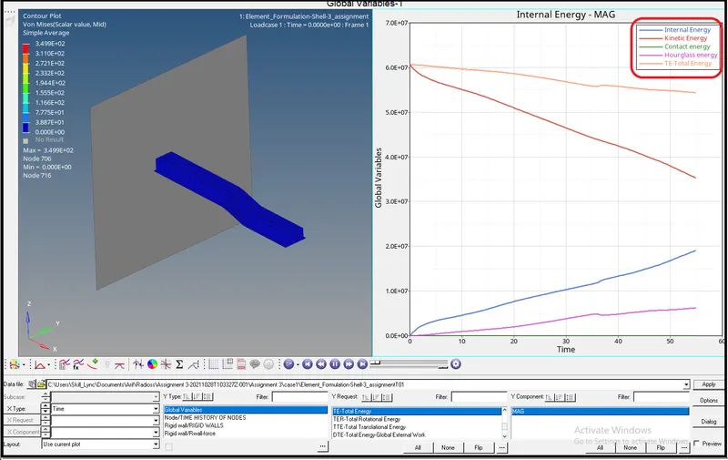
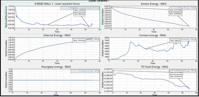
• This graph is represenation of combined all energies togather.
• Now we will see and analyize each indivisual energies.

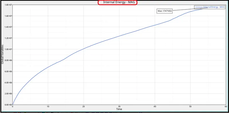
1. Internal Energy-

Graph-

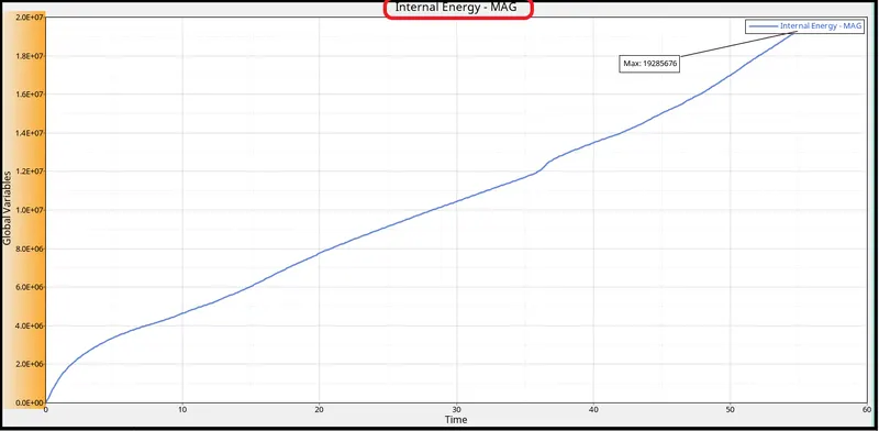
• According to graph as we can see that the internal energy at t=0 is zero.
• Because as we know internal enery is combination of heat interaction and work done,

IE=Q±W here Q=0 and W=Fxd where d is displacement

since at t=0 d=0

so, W=0

So at t=0, IE=0

• And then it will gradually increase as the deformation takes placed due to mass and velocity is given at one end.
• Due to mass and velocity Kinetic energy will also produce.

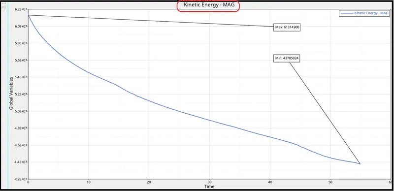
Kinetic Enrgy-

Graph-

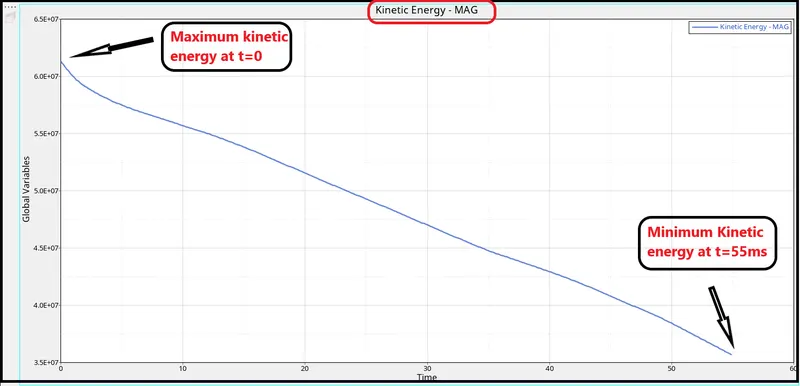
• As we know the formula of kinetic energy is KE=1/2 m v²

Unit= kg m² / s²

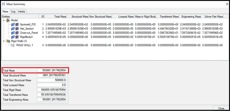
Now check for mass and velocity at t=0

Mass

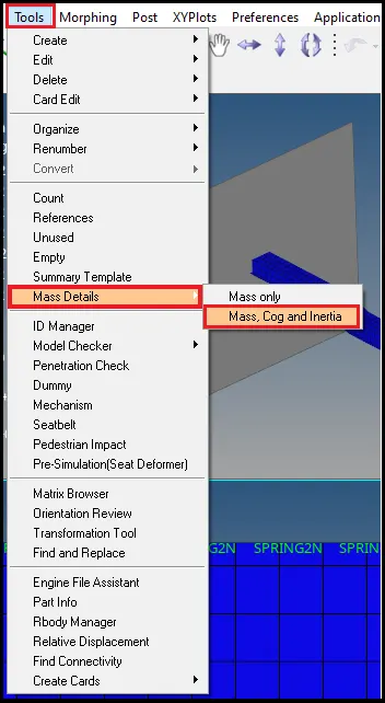
• Velocity-

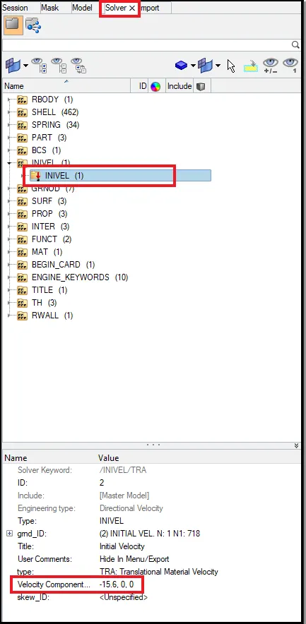
• Now we have checked the mass and velocity values.

Kinetic energy calculation-

KE= 1/2 m v²

= 1/2 x (503881.28179) x (-15.60)^2

= 61312274.38 kg m² / s²

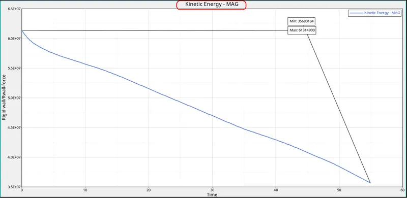
• This calculated energy is at t=0 and after this time kinetic energy start decreasing continuesly as shown in grapgh.
• It will decrease just beacuse of decease in velocity after initial moment.Since rail start deforming so energies start restoring.
• And at the end of deformation the velocity becomes zero at that point kinetic energy achive their lower value.

Contact Energy-

Graph-

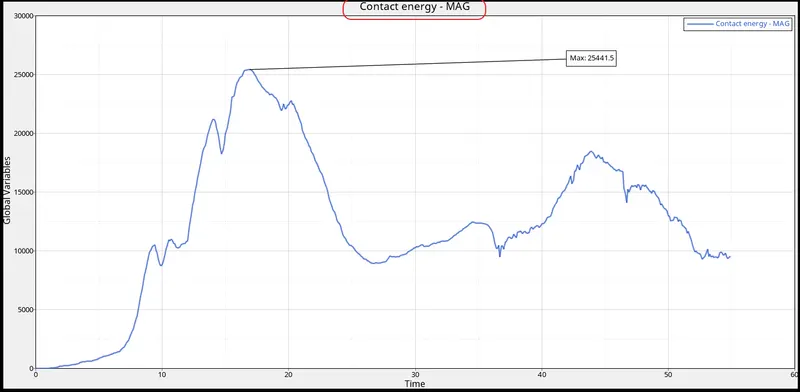
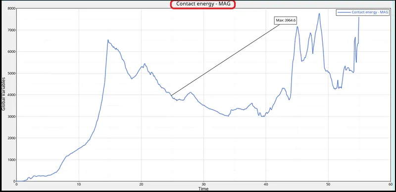
• At t=0 contact energy is zero because at that point thre is no contact of rail to the rigid wall.
• As the velocity given to the rail it starts deforming and gets into contact to rigid wall then contact energy starts getting increases continuously after that time.
• During deformation, rail elements are getting into contact with each other due to that contact energy is generated.
• And in between some energy start storing in deformation so that contact energy start decreasing also.
• This energy we get due to crash of rail to the rigid wall so some amount if contact enery will be generate.

Hourglass energy-

Graph-

Total Energy-

Graph-

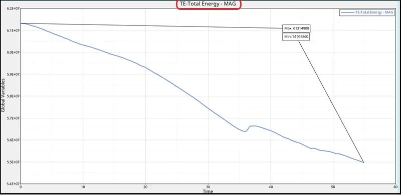
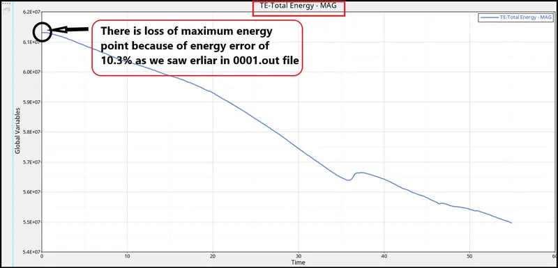
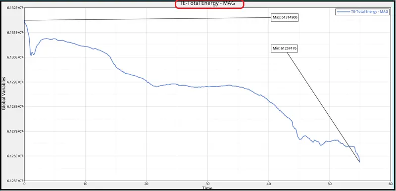
• Since we know that total energy is sum of kinetic energy, Internal energy, Contact energy, Hourglass energy.
• At time t=0 there is only one kind of energy is present is kinetic energy so,

Total energy at t=0 is equal to kinetic energy at t=0

Total energy(at t=0) = 61312274.34 kg m² / s²

• By the time it will decrease as shown in figure due to energy error.

Energy error is 10.3%

Claculate Total energy at t=55 ms

Since energy decreases by 10.3%

10.3% of 61312274.34 =(10.3/100)x 61312274.34

= 6315164.26 amount of loss

Total energy at (t=55 ms) = Total energy (at t=0) − Loss of energy

=61312274.34 − 6315164.26

Total energy at (t=55 ms) =54997110.078

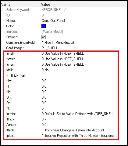
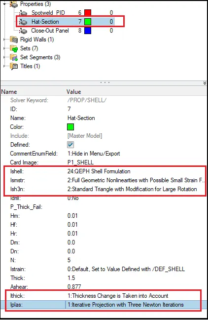
Case-2 Assign recomended prameter to property card-

Hat section property-

Close out panel property-

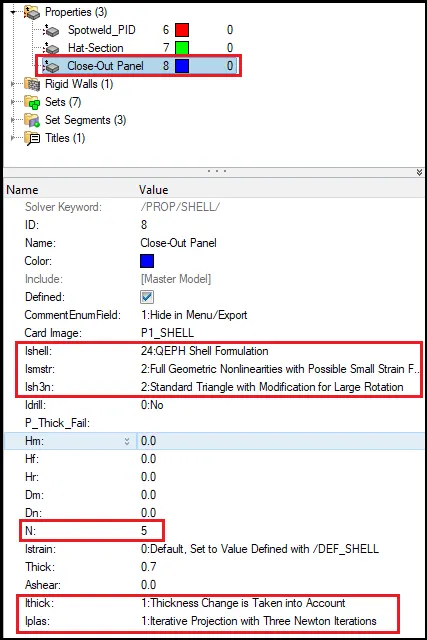
• Now follow the same procedure fo engine file edit as we did for case-1.
• And then run the model.

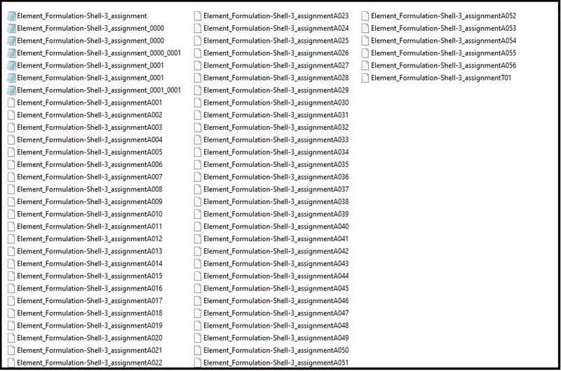
• After running the solver we get all 56 file.

Now check for energy error-

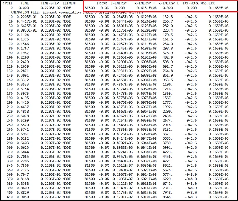
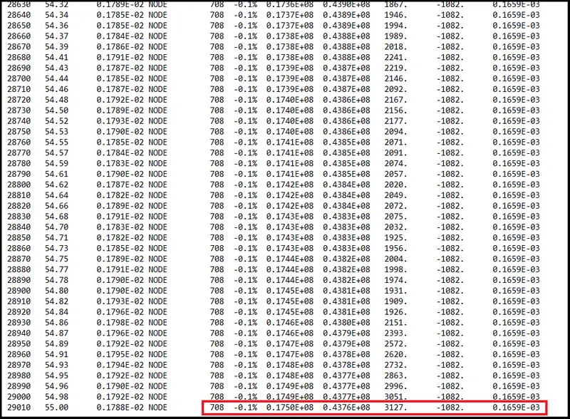
Fig-Engine file(0001.out)

• we can see after assigning the elemental parameter to property card we can see that errors are reduced.
• Now we will check the energy graphs for updated parameter case.

Simulation in Hyperview-

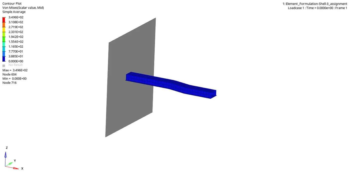
Energy graphs in Hypergraph 2D-

Rigid wall forces-

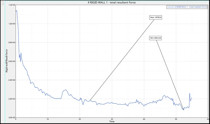
• Here in case-2 we can see that a slight improvement in energy curve because we have used recomended shell parameters.
• Since we used QEPH (Ishell 24) which is improved integerated nodes,due to this now hourglass energy found so that loss of energies are less and added to total energy.

Kinetic Energy-

Internal Energy-

Contact Energy

Hourglass Energy-

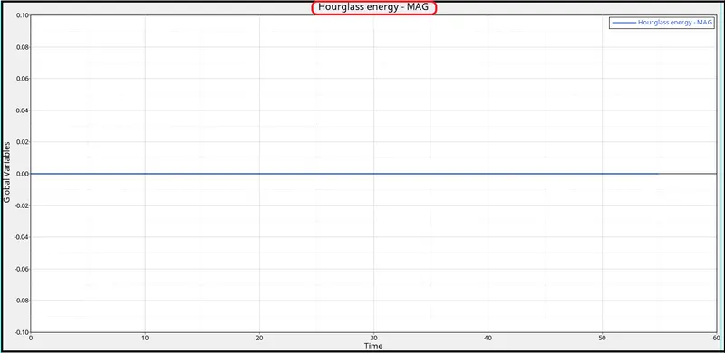
• Here as we can see hourglass energy is constant cause we have used (QEPH Ishell24).
• It is an improved under-integerated 4 node element, so no hourglass happened.

Total Energy-

All Graph combined-

Result-

• Run time and amination file is updated in solver file.
• Simulation has been runned without assigning recomended parameters.
• Graph are plotted for case-1.
• Simulation has bessn runned with assigning recomended parameters.
• For 2nd case also graphs are plotted and both cases are compared in terms of energy variation.

Conclusion and Larning outcome-

• In this assignment i learn the engine file creation for simulation run.
• Thne how to perform postprocessing like plotting graphs for energies.
• And also how to see the animation of simulation in hyperview.
• Then How to assign the recomended parameters and understand their benifit in controling hourglass.
• How to check the graph variation for both the cases and conclude the better one.
• From this assignment according to me simulation with assigning the thickness is better choice which is case-2.