2D diffusion equation using matlab

clear all
close all
clc

%% Defining the Mesh
n_points = 50;
dom_size = 1;
h = dom_size/(n_points - 1);
dt = 0.0001;
alpha = dt/(h*h);

%% Initializing the problem
y(n_points, n_points) = 0;
y(1,:) = 1;

y_new(n_points , n_points) = 0;
y_new(1,:) = 1;

error_mag = 1;
error_req = 1e-6;
iterations = 0;

%% Tracking the error magnitude
error_track = 0;

 %%Calculations

while error_mag > error_req
    for i = 2:(n_points - 1);
        for j = 2:(n_points - 1);
            y_new(i,j) = y(i,j)+ alpha.*(y(i-1,j)+ y(i+1,j) + y(i,j-1) + y(i,j+1) - 4*y(i,j));
        end
    end
    
    iterations = iterations +1;
    
    %% calculation of error magnitude
    
    error_mag = 0;
    
    for i = 2:(n_points - 1);
        for j = 2:(n_points - 1);
            error_mag = error_mag + abs(y(i,j) - y_new(i,j));
            error_track(iterations) = error_mag;
        end
    end
    if rem(iterations, 1000) == 0;
        iterations
        error_mag
    end
    
    % Assigning old to New
    
    y = y_new;
end

%% Plotting

x_dom = ((1:n_points)-1).*h;
y_dom = 1-((1:n_points)-1).*h;
[X,Y] = meshgrid(x_dom,y_dom);
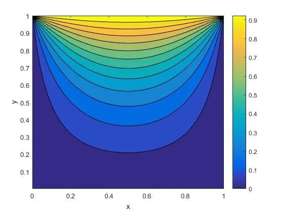
contourf(X,Y,y,12);
colorbar

xlabel('x');
ylabel('y');
%print(gcf,'Example.png','-dpng','-r300');


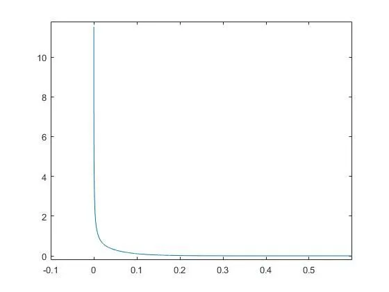
%Plot the error with time

figure;
time =  dt.*(1:iterations);
plot(time, error_track)

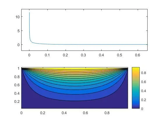
% concept of sub plots

figure;
subplot(2,1,1);
plot(time,error_track);
subplot(2,1,2)
contourf(X,Y,y,12);
colorbar

Results

iterations =

        1000


error_mag =

    0.1081


iterations =

        2000


error_mag =

    0.0150


iterations =

        3000


error_mag =

    0.0021


iterations =

        4000


error_mag =

   2.8846e-04


iterations =

        5000


error_mag =

   4.0020e-05


iterations =

        6000


error_mag =

   5.5521e-06