Matrix Based Implicit Solution of Steady Diffusion Equation

clear all
close all
clc

%% Getting the inputs sorted out

% Total Number of Grid Points
N = 5;
% Domain length
L = 0.5;
% Grid spacing
h = (L/N);
% Spacial location (for exact soltion)
x = 0:0.001:L;
% Thermal conductivity
k = 1000;
% Area
A = 10*10^-3;
% Boundary conditions
T_a = 100;
T_b = 500;

% initializing the tempetature
T(N) = 500;
T(1) = 100;


%% Forming the matrices

C(N,N) = 0;
D(N) = 0;

for i = 1:N
    if i > 1 && i < N
        C(i,i) = 2*k*A/h; %a_p
        C(i,i-1) = -k*A/h; %-a_w
        C(i,i+1) = -k*A/h; %-a_e
        D(i) = 0;
        
    elseif i==1 %Left boundary
        C(i,i) = 3*k*A/h;
        C(i,i+1) = -k*A/h;
        D(i) = 2*k*(A/h)*T_a;
    else %right boundary
        C(i,i) = 3*k*A/h;
        C(i,i-1) = -k*A/h;
        D(i) = 2*k*(A/h)*T_b;
    end
end

% Obtaining the solution

T = CD';

%% Plotting
% Spacial location of the grid points
x_g = h/2:h:(N)*h;
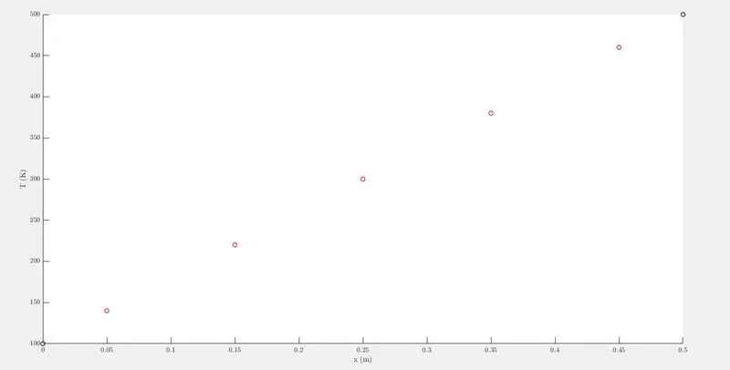
figure(1);
hold on
plot(x_g, T,'ro', 'Linewidth', 1) % Numerical Solution
plot([0 , L], [T_a, T_b], 'ko','Linewidth', 1) % Boundary values
xlabel('x (m)', 'interpret', 'Latex');
ylabel('T (K)', 'interpret', 'Latex');
set(gca, 'TicklabelInterpreter', 'Latex')
yticks([100:100:500]);