Write a code to fit a curve of the original Data set using MATLAB
Week3 Report.
- Aim: To write a code to fit a curve of the given data set and to use the splitwise method for the same.
- Introduction: Curve fitting is the process of constructing a curve, or mathematical function, that has the best fit to a series of data points, possibly subject to constraints. Curve fitting can involve either interpolation, where an exact fit to the data is required, or smoothing,in which a "smooth" function is constructed that approximately fits the data. A related topic is regression analysis, which focuses more on questions of statistical inference such as how much uncertainty is present in a curve that is fit to data observed with random errors. Fitted curves can be used as an aid for data visualization, to infer values of a function where no data are available, and to summarize the relationships among two or more variables. Extrapolation refers to the use of a fitted curve beyond the range of the observed data, and is subject to a degree of uncertainty since it may reflect the method used to construct the curve as much as it reflects the observed data.
We know,Curve fitting is one of the most powerful and most widely used analysis tools in Origin. Curve fitting examines the relationship between one or more predictors (independent variables) and a response variable (dependent variable), with the goal of defining a "best fit" model of the relationship. Origin provides tools for linear, polynomial, and nonlinear curve fitting along with validation and goodness-of-fit tests. You can summarize and present your results with customized fitting reports. There are many time-saving options such as a copy-and-paste-operation feature which allows you to "paste" a just-completed fitting operation to another curve or data column. Curve fitting operations can also be part of an Analysis Template, allowing you to perform batch fitting operations on any number of data files or data columns.
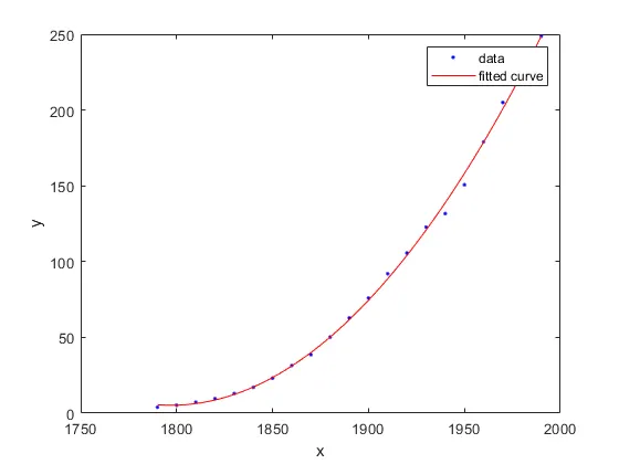
Example of a Curve-Fit - Code/Logic:
1. We firstly need to clear and close all the previously entered codes and the present values of the already used variables, hence we use the following commands:
clear all
close all
clc
2. In the next step, we can use the Load command to load the file that stores the Specific Heats at different Temperatures. After we load this file, we then assign the variable of 'temperature' to the first column and the variable of 'cp' to the second column.
3. After we have defined the temperatures and the Specific heat for the given data, we then calculate the coefficients by using the polyfit command and use the polyval command to get the predicted Specific Heats as well.
4. In the next step, we will plot the original Data set Curve and the curve fit in one tab. We must ensure that we are using the first order of polynomial and in the next step, we will use the same set of codes, but we will just change the order of the polynomiial to three. By doing this, we can comparebetween two curves that we get.
5. We must use a new figure tab to view the curve with respect to the original Data Set curve. Hence, we use the Figure (2) command before we write the next set of codes to get a third Degree of curve fit. We can also use the xlabel and ylabel command to label the X-Axis and the Y-Axis respectively. In our case, we have labelled them as Temperature [K] and Specific Heat [KJ / Kmol-K] at the x and y axis respectively.
6. In the next step, we have simply calculated the goodness of the curve fit that we have done. To understand the goodness of the curve, we must calculate the following four parameters:
a. SSE - Sum of Squares due to error.
b. R - Relation between the response values and the predicted values.
c. R_adj - Adjusted Value of R.
d. RMSE - Root Mean Squared Error.
To calculate the SSE,
a. `SSE ("sum of squared errors") = sum_(i=1)^n"Error(i)"^2`
Hence,
`SSR = sum_(i=1)^n(f(x(i))-Mean)^2`
`SSE = sum_(i=1)^n(Y(i)-f(x(i)))^2`
We know that SST is the summation of SSR and SSE, so:
`SST=SSR+SSE`
b. From these two values we can calculate the `R^2` value as the following:
`R^2 = (SSR)/(SST)`
c. To caculate the R_Adj value, we can use the following formula: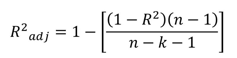
where, n: total number of Data points and,
k: Number of independent Variables
d. To calculate the RMSE Value, we can use either of the formulae:
`RMSE = sqrt((sum_(i=1)^n(Y(i)-f(x(i)))^2)/n) = sqrt((SSE)/n)`
Using the above Formulae, we can then calculate the Goodness of the curves for all the cases. The code is given below.
The Code for the Linear and Cubic Polynomial is as follows:
clear all close all clc %Preparing Data cp_data = load ('data'); temperature = cp_data(:,1); cp = cp_data (:,2); %Curve fit for a Linear Polynomial %cp = a*T + b co_effs = polyfit(temperature , cp , 1); %1 is the degree of the polynomial predicted_cp1 = polyval(co_effs, temperature); %compare curvefit and the original data plot (temperature, cp, 'linewidth', 2) hold on plot(temperature, predicted_cp1, 'linewidth' , 2, 'color', 'r') xlabel('Temperature [K]') ylabel('Specific Heat [KJ/Kmol-K]') legend ('Original Dataset', 'Curvefit') figure (2) %Curve fit for a Linear Polynomial %cp = a*T^3 + b*T^2 + c*T + d co_effs = polyfit (temperature , cp , 3); %3 is the degree of the polynomial predicted_cp2 = polyval (co_effs, temperature); %compare curvefit and the original data plot (temperature, cp, 'linewidth', 2) hold on plot(temperature, predicted_cp2, 'linewidth' , 2, 'color', 'r') xlabel('Temperature [K]') ylabel('Specific Heat [KJ/Kmol-K]') legend ('Original Dataset', 'Curvefit') %Calculating the Goodness of the curvefit using Polynomial Degree = 1 i= 1:3200; m1= mean(predicted_cp1); x1(i) = predicted_cp1(i) - m1; y1(i) = cp(i) - predicted_cp1(i); SSR1 = sum (x1(i).^2); SSE1 = sum (y1(i).^2); SST1 = SSR1 + SSE1; R1 = sqrt (SSR1/SST1) %To measure the Adjusted R-Square n = 3200; %Number of Datapoints k = 1; %Number of Independent Variables R_Adj1 = sqrt(1 - ((1-R1^2)*(n-1) / (n-k-1))) %To measure Root Mean Squared error RMSE1 = sqrt(SSE1 / n) %Calculating the Goodness of the curvefit using Polynomial Degree = 3 i= 1:3200; m2= mean(predicted_cp2); x2(i) = predicted_cp2(i) - m2; y2(i) = cp(i) - predicted_cp2(i); SSR2 = sum (x2(i).^2); SSE2 = sum (y2(i).^2); SST2 = SSR2 + SSE2; R2 = sqrt (SSR2/SST2) %To measure the Adjusted R-Square n = 3200; %Number of Datapoints k = 1; %Number of Independent Variables R_Adj2 = sqrt(1 - ((1-R2^2)*(n-1) / (n-k-1))) %To measure Root Mean Squared error RMSE2 = sqrt(SSE2 / n)
We can see that, we have calculated the goodness of the curve when we use both the curves, i.e The linear polynomial and the Cubic Polynomial for the curve fit.
For the Linear Polynomial we get a value of R = 0.9617 and the value of RMSE = 25.991
For the Cubic Polynomial, we get a value of R = 0.9984 and the value of RMSE = 5.427
As the Value of R is much near to 1 and the value of RMSE is also much lesser in the case of the cubic polynomial, we can conclude that it gives a much better curve fit than the Linear type Polynomial.
Using the Splitwise method:
1. In this method, we basically split the entire original dataset curve into a bunch of small curves so that we can get a much more accurate curve by using a smaller degree of polynomial.
2. Another reason for using the splitwise method is that we can reduce the sensitivity of the output change with respect to the inputs given.
3. In this method, we simply divide all the Temperature and Specific heat values into seperate Arrays and then use a set of codes to plot the graph for a Quadratic degree of polynomial.
The Code for the Splitwise method is as follows:
clear all close all clc %Splitwise Method. %Preparing Data cp_data = load('data'); temperature = cp_data(:,1); cp = cp_data (:,2); %Dividing the temperature values t1 = temperature(1:800); t2 = temperature(801:1600); t3 = temperature(1601:2400); t4 = temperature(2401:3200); Temperature = [t1; t2; t3; t4]; %Dividing the Specific Heat Values cp1 = cp(1:800); cp2 = cp(801:1600); cp3 = cp(1601:2400); cp4 = cp(2401:3200); CP = [cp1; cp2; cp3; cp4]; %Curvefit for a Second Order Polynomial co_effs1 = polyfit (t1 , cp1 , 2.0); %2 is the degree of the polynomial predicted_cp1 = polyval(co_effs1, t1); co_effs2 = polyfit(t2 , cp2 , 2.0); predicted_cp2 = polyval(co_effs2, t2); co_effs3 = polyfit(t3 , cp3 , 2.0); predicted_cp3 = polyval(co_effs3, t3); co_effs4 = polyfit(t4 , cp4 , 2.0); predicted_cp4 = polyval(co_effs4, t4); Predicted_CP = [predicted_cp1; predicted_cp2; predicted_cp3; predicted_cp4]; %Comparing curvefit and the Original Data plot (temperature, cp, 'linewidth', 3, 'color', 'b') hold on plot(Temperature,Predicted_CP, 'linewidth' , 1.5, 'color', 'r') xlabel('Temperature [K]') ylabel('Specific Heat [KJ/Kmol-K]') legend ('Original Dataset', 'Curvefit') %Calculating the Goodness of the curvefit using the Splitwise method. i= 1:3200; m = mean(Predicted_CP); x(i) = Predicted_CP(i) - m; y(i) = CP(i) - Predicted_CP(i) SSR = sum (x(i).^2); SSE = sum (y(i).^2); SST = SSR + SSE; R = sqrt(SSR/SST) %To measure the Adjusted R-Square n = 3200; %Number of Datapoints k = 1; %Number of Independent Variables R_Adj = sqrt(1 - ((1-R^2)*(n-1) / (n-k-1))) %To measure Root Mean Squared error RMSE = sqrt(SSE / n)
The values for R in this case is approximately = 0.9999 and the value of RMSE is = 1.2203 in this case. This just shows that we get a higher accuracy curve fit for a smaller degree of the polynomial used. - Body of Content:
Q1. How to make a curve fit perfectly?
- A curve can be said to be perfectly fit if the error between the calculated and the original Data set is zero or negligible. We can use the method of Interpolation to get a near perfect curve fit. Another method that can be used is to do the centering and Scaling.
Q2.How to get the best fit?
- We understand that there is a difference between the perfect fit and the best fit of curve. In perfect fit, the Error with respect to the original data set is zero, but whereas in best fit, the Error is to be kept as minimum as possible. The values of `R^2`in perfect fit is 1 and in the case of best fit, the values can range from 0.95 to 1.0.
We can get the Best fit by using the following:
a. The sum of Squares due to error
b. R-Square
c. R-Square Adjusted
d. Root Mean Squared Error (RMSE)
Q3. What could be done to improve the cubic fit?
- One of the ways to improve a cubic fit is to use the Splitwise method. And in this method, the more number of divisions we make to the data, the higher the accuracy of the curve fit will be. The main advantage of this method is that as the degree of the polynomial increases, the sensitivity of the output change also increases with respect to the input, and this problem is taken care of in the Splitwise method.
We can even use a quartic degree(order four) of polynomial as well. - Results:
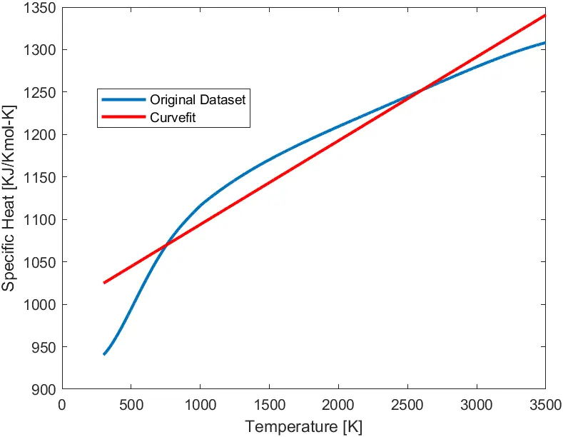
Linear Polynomial Curve Fit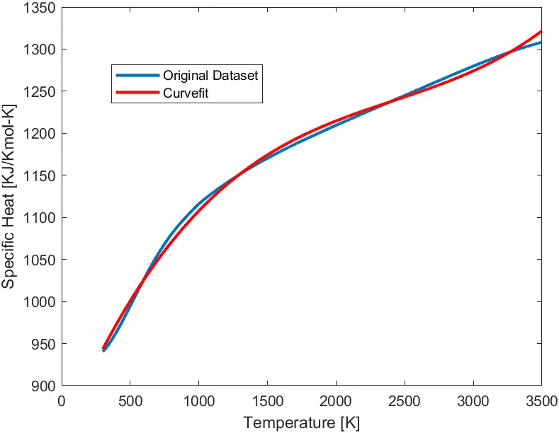
Cubic Polynomial Curve Fit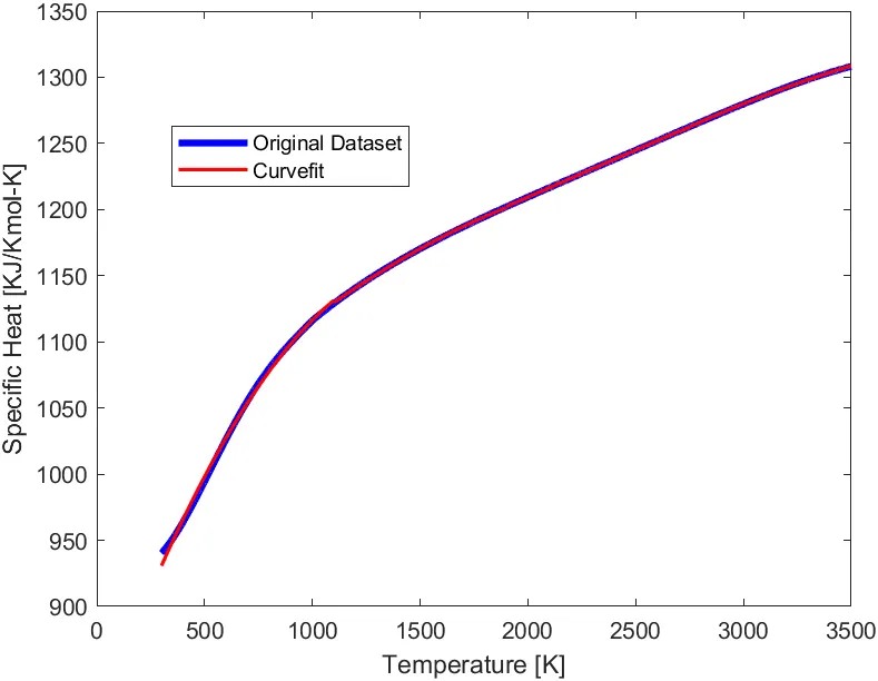
Splitwise Method Curve Fit (We use a Quadratic Degree of Polynomial) - Errors: The errors that I faced were majorly the typos and the parantheses while using specific commands. So, when MATLAB pointed out an error, I checked for the line number and then checked for any typos and corrected them right away.
Another Error that I faced during this coding is the use of commas and semi-colons when forming an array. So, when we make an array from a pre-existing set of values, then we must use the semi-colon instead of the commas, as it forms a matrix and not an Array as we want. - Conclusion: In conclusion, I would like to state that, this challenge helped me understand how to perform a Curve Fit for a given data set. I even understood the Splitwise method for curve fitting and how to calculate the Goodness of a curvefit as well.