Week 9- Unsteady moving zones Approach

Aim- To study and simulate the turbomachinery component using an unsteady state approach and for the moving zones we go with the "Moving Mesh Formulation Approach".

Objective-

• Simulate the Moving Mesh Approach on the turbomachinery component.
• Explain the moving mesh approach and why we considered it.
• The rotational speed of the blade is 300rpm.

Theory-

The moving Mesh Formulation approach is a simulation approach in fluent for the moving of the mesh along the geometry, it generates a new mesh for every timestep.

The moving Mesh Approach is used for the Unsteady Phenomenon, and when we have a rotating wall that will change the skewness of your element.

Used for Modelling Unsteady Phenomenon such as

• Vortex Induced Flows
• Interaction of Vortex with bodies
• Mesh is moving
• Topology Changes with Time
• Control Volume Changes with Time
• Unsteady Phenomenon
• If Unsteadiness is important

Setup-

• For the simulation in fluent directly import the mesh file on the Ansys fluent name domain 1, and use the 'append' tool to add Domain 2 and Domain 3.
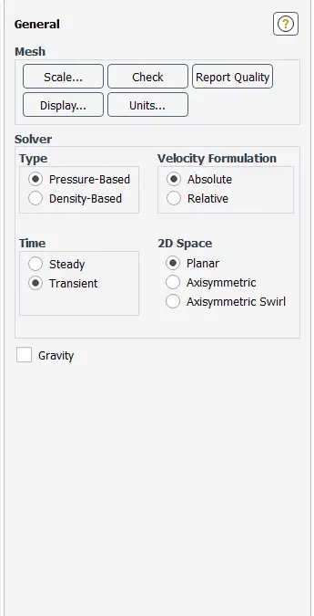
• For the simulation, we go with,

Transient State Analysis

Type - Pressure Based

2d surface - planar

velocity formulation - Absolute

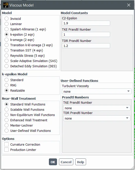
• For the viscous model,

K-epsilon model- Realizable- Standard wall function

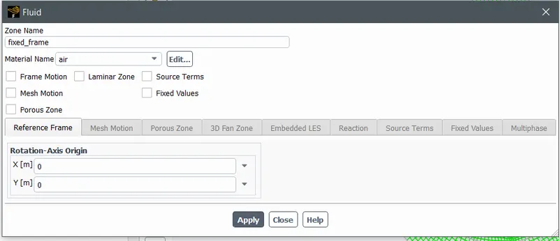
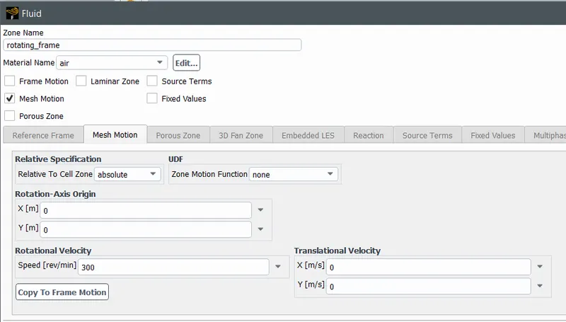
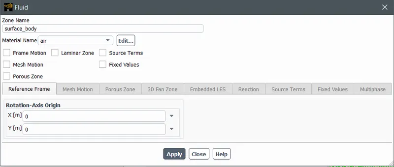
• Cell Zone Conditions

Fixed Frame - Fluid

Rotating Frame - Fluid

Mesh Motion

Speed(rev/min)- 300

Surface Body - Fluid

• Boundary Conditions-

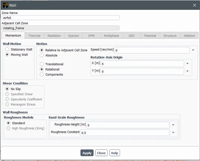
Airfoil- Wall = Moving wall - Rotational

Relative to adjacent cell zones

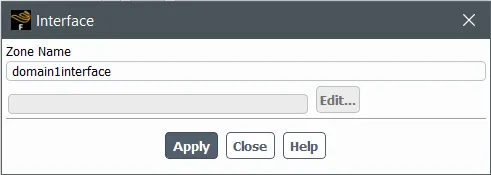
Domain1_Interface = Interface

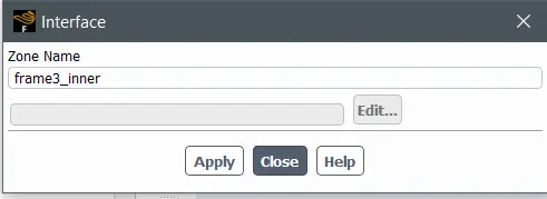
Frame3_Inner = Interface

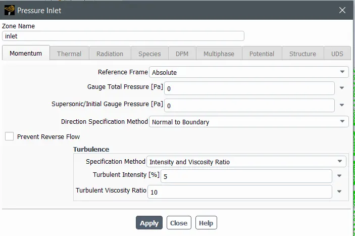
Inlet = Pressure Inlet(0 pascal)

Outlet = Pressure Outlet

Rotating Domain_inner = Interface

Rotating Domain_outer = Interface

Wall = wall

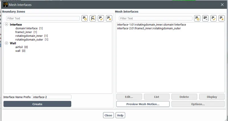
• Mesh-Interface -

Interface-1 = Domain1_Interface + Rotating Domain_inner

Interface-2 = Frame3_Inner + Rotating Domain_outer

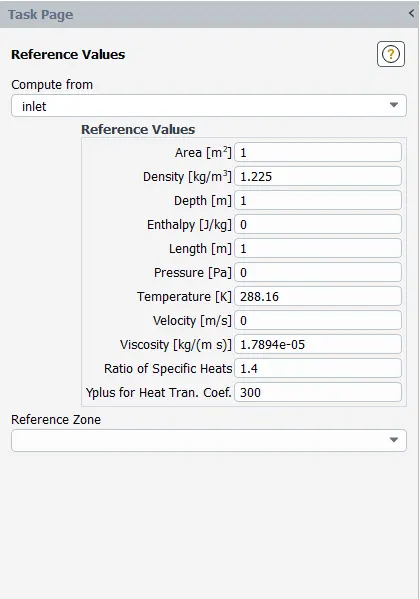
• Reference values = Compute from INLET

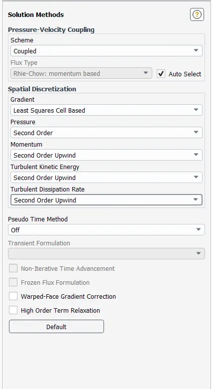
• Solution Methods = coupled scheme with Second Order upwind

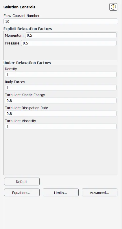
• Courant Number = 10

• Report - Flux Report(Mass Flow Rate)= outlet
• XY Plot - New surface - Line/rake = X(m)=0,X(m)= 1.5
• Run Calculation

Number of time steps- 1000(Note we ran this simulation twice)

Time step size - 0.0002

Max Iterations/Time step - 100

Results-

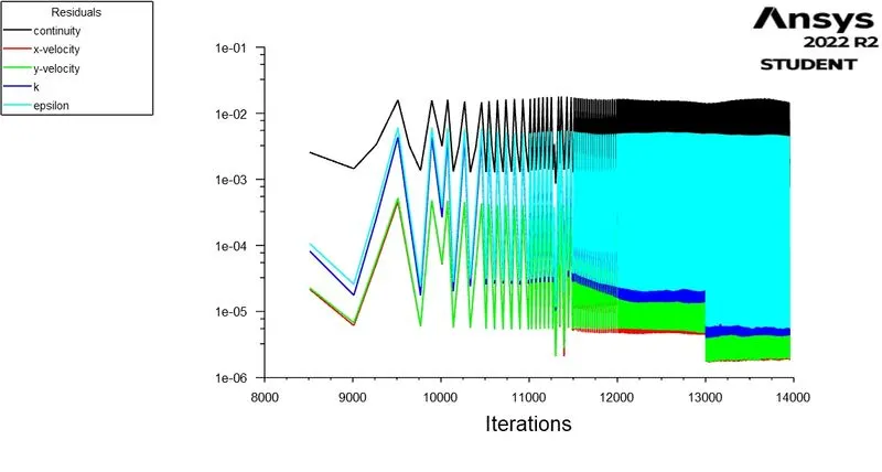
We ran this simulation for 14000 Iterations and stable result is obtained.

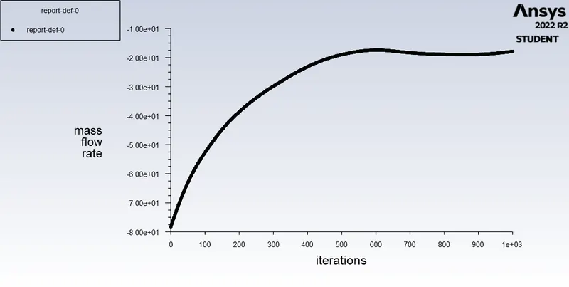
The mass flow rate at the Outlet is -17.884 Kg/m^3, a -ve sign because the fluid is leaving the domain.

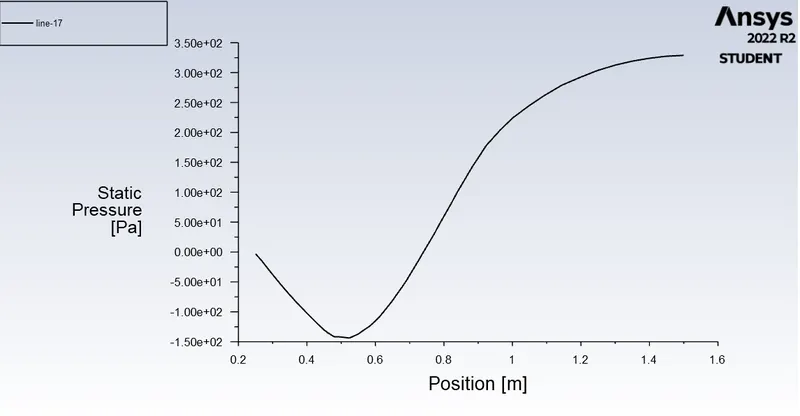
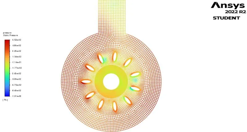
The maximum pressure is around 633 Pa and the minimum pressure is around 614 Pa. Most regions have higher pressure due to the accumulation of air as the blades rotate, and the inlet and outlet have low pressures due to the existence of boundary conditions.

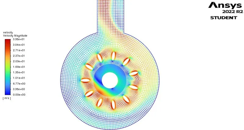
The maximum velocity is around 33.28 m/s, seen near the blades. This is expected as the airfoils rotate, due to flow separation and accumulation the velocity of fluid increases.

The contour also shows the path taken by air into the outlet pipe, and it is seen that most of the space in the domain actually has low to very low magnitudes of velocity.

Conclusion-

A moving Mesh Approach is Performed on the turbomachinery as mentioned and all the parameters have been captured for achieving the values of velocity, pressure and mass flow rate around the airfoil.

The moving mesh Approach needs more computational power and time to achieve the solution converged than the Moving Reference Frame Approach. More accurate results is been achieved using Mesh using

Moving Mesh Approach.