Week 9 - Senstivity Analysis Assignment
Use the source code as shown in the video, but alter it to satisfy the following conditions
- Write a code that takes all the reactions from the GRI mechanism and calculates 10 most sensitive reactions
- The sensitivity parameter should be with respect to the Temperature (It should find the sensitivity with respect to the temperature not 'OH' as shown in the video)
- Consider the initial conditions as shown in the video
- Your program should show the reaction strings in the order of greatest sensitivity to the least sensitivity
The sensitivity of a paramtere with respect to the reaction is defined by the equation:
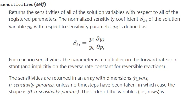
Sensitivity defines how a specific variable is sensitvie to the specific equation.
The code strucure:
- Declaring the header file i.e. the importing the libraries required
- decalring the variable gas which is the instance of the class cantera
- declaring the temp, pressure and the moles of the composition of the gas
- declaring the reactor to be ideal gas const pressure of the obj gas
- creating the reactor net for the reactor object
- creating arrays to store the reaction and the number of reactions in the gri30 mechanism
- For loop to store the add the sensitivities to the reactor object
- Setting up tight tolerances for simulation and the sensitivity variable s
- writing an for loop to iterate over all the time steps to store the gradients and append the states i.e solution Array for all the time stamps
- Storing all the sensitivities that are more sensitive through out all the simlation i.e. over all the time steps
- Use the SORT and ZIP command to pair the variables and sort them and store them in an another arrays by unzipping them
- Finaly making the subplot and the bar graph
the code is as follows:
"""
PART I
Use the same reactor network code as shown in the video to evaluate the sensitivities of a simulation
 (simulation time = 10 secs)

Write a code that takes all the reactions from the GRI mechanism and calculates 10 most sensitive reactions
The sensitivity parameter should be with respect to the Temperature (It should find the sensitivity with respect to the temperature not 'OH' as shown in the video
Consider the initial conditions as shown in the video
Your program should show the reaction strings in the order of greatest sensitivity to the least sensitivity
"""
import numpy as np
import matplotlib.pyplot as plt
import cantera as cnt
# Logic I AM TRYING BY CREATING AN FUNCTION FILE

gas =cnt.Solution('gri30.yaml')
temp=1500
pres=cnt.one_atm

gas.TPX=temp, pres, {'CH4':1, 'N2':7.52, 'O2': 2}
Reactor=cnt.IdealGasConstPressureReactor(gas, name='R1')
Simulation=cnt.ReactorNet([Reactor])

"""
property reaction_equations
Returns a list containing the reaction equation for all reactions in the mechanism
(if indices is unspecified) or the equations for each reaction in the sequence indices.
"""
reactions_Eq=gas.reaction_equations()

"""
property n_reactions
Number of reactions in the reaction mechanism.
"""
no_reactions_mech=gas.n_reactions

# Top 10 sensitivities are demanded in the problem statement
No_sensitivities_demanded=10


# Enabling the sensitivity with respect to the rates of all the reactions to the Reactor
for i in range(no_reactions_mech):
	Reactor.add_sensitivity_reaction(i)

# Settting up the tolerances for the solution and for the sensitivities

Simulation.rtol=1e-05
Simulation.atol=1e-15

Simulation.rtol_sensitivity=1e-06
Simulation.atol_sensitivity=1e-06

col=np.arange(0, 2e-03, 5e-06)

sensitivity_temp=[0]*no_reactions_mech

states=cnt.SolutionArray(gas, extra=['time'])
reactions_num=np.arange(1, no_reactions_mech+1)

# Time loop begins here
for t in np.arange(0, 2e-03, 5e-06):

	Simulation.advance(t)
	states.append(Reactor.thermo.state, time=t*1e+03)

	for j in range(no_reactions_mech):
		gradient=Simulation.sensitivity('temperature', j)

		if abs(gradient) >= abs(sensitivity_temp[j]):

			sensitivity_temp[j]=gradient

# Sorting the reactions and sensitivites based on the values of the sensitiviteis

print(np.shape(sensitivity_temp))


## Usign the logic of ZIP along with the sorted we will try to figure out the first 10 reactions with highest sensitivities
# For more info use: https://www.kite.com/python/answers/how-to-sort-two-lists-together-in-python

Zipped_pair=sorted(zip(np.abs(sensitivity_temp),reactions_Eq, reactions_num, sensitivity_temp), reverse=True)
max_Sensi, max_reactions, max_reac_num, act_sensi_temp=zip(*Zipped_pair)
#sensitivity_temp, reactions_Eq, reactions_num= [list[tup] for tup in tup]

########################################### Plotting commands begins here#####################################################################
fig, ((ax1, ax2), (ax3, ax4)) = plt.subplots(2, 2)
fig.suptitle('variation of the parameters with time')

ax1.plot(states.time, states.T)
ax1.set_xlabel(xlabel='time')
ax1.set_ylabel(ylabel='Temperature')
ax1.set_title("Variation of temperature with time")
ax1.grid()

ax2.plot(states.time, states('CH4').X)
ax2.set_xlabel(xlabel='time')
ax2.set_ylabel(ylabel='mole_fraction_CH4')
ax2.set_title("CH4 Variation with time")
ax2.grid()

ax3.plot(states.time, states('OH').X)
ax3.set_xlabel(xlabel='time')
ax3.set_ylabel(ylabel='mole_fraction_OH')
ax3.set_title("OH Variation with time")
ax3.grid()

ax4.plot(states.time, states('H').X)
ax4.set_xlabel(xlabel='time')
ax4.set_ylabel(ylabel='mole_fraction_H')
ax4.set_title("H Variation with time")
ax4.grid()

fig.tight_layout()
fig.show()

#### Bar graphh to present the top 10 sensitivities and their reactions##############################
plt.figure(2)
plt.barh(max_reactions[0:10], act_sensi_temp[0:10], color='red')
plt.xlabel('sensitivity')
plt.ylabel('Reactions')
plt.title('Top 10 temperature sensitive reactions')
plt.gca().invert_yaxis()
plt.grid()
plt.tight_layout()
plt.show()
The output is as follows:
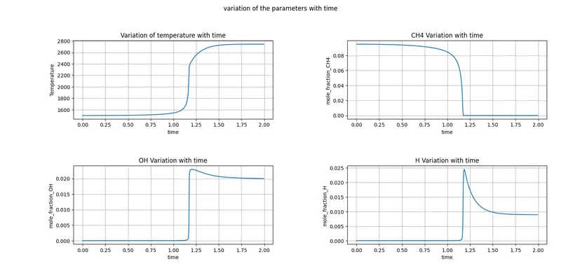
From the figure it can be observed that the temperature max at 1.125 sec where the auto ignition happens and the combustion begins in the reactor. It can further be seen that the reactant i.e. CH$ mole fraction decreases from 2 to 0 indicating the complete comsumption og reactiant.
It can also be seen that the variation of OH and H are increaing as they are products and there mole fraction will grow over time and finally come to an saturated value.
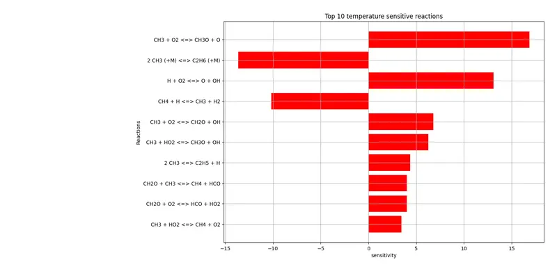
From the graph it can be intrepereted tha: for the reactions 7 and 9 the reaction rate are negative and for these reactions, i.e. with ncrease in the reactions over the time the ignition delay will incease. For all other reactions it's vice versa.
For additional points plot a graph of sensitivities vs the reactions as shown in the sensitivity theory video.
The above code is added with few more additional lines at : 59 60, 73 and 74. The code is asl follows:
"""
PART I
Use the same reactor network code as shown in the video to evaluate the sensitivities of a simulation
 (simulation time = 10 secs)

Write a code that takes all the reactions from the GRI mechanism and calculates 10 most sensitive reactions
The sensitivity parameter should be with respect to the Temperature (It should find the sensitivity with respect to the temperature not 'OH' as shown in the video
Consider the initial conditions as shown in the video
Your program should show the reaction strings in the order of greatest sensitivity to the least sensitivity
"""
import numpy as np
import matplotlib.pyplot as plt
import cantera as cnt
# Logic I AM TRYING BY CREATING AN FUNCTION FILE

gas =cnt.Solution('gri30.yaml')
temp=1500
pres=cnt.one_atm

gas.TPX=temp, pres, {'CH4':1, 'N2':7.52, 'O2': 2}
Reactor=cnt.IdealGasConstPressureReactor(gas, name='R1')
Simulation=cnt.ReactorNet([Reactor])

"""
property reaction_equations
Returns a list containing the reaction equation for all reactions in the mechanism
(if indices is unspecified) or the equations for each reaction in the sequence indices.
"""
reactions_Eq=gas.reaction_equations()

"""
property n_reactions
Number of reactions in the reaction mechanism.
"""
no_reactions_mech=gas.n_reactions

# Top 10 sensitivities are demanded in the problem statement
No_sensitivities_demanded=10


# Enabling the sensitivity with respect to the rates of all the reactions to the Reactor
for i in range(no_reactions_mech):
	Reactor.add_sensitivity_reaction(i)

# Settting up the tolerances for the solution and for the sensitivities

Simulation.rtol=1e-05
Simulation.atol=1e-15

Simulation.rtol_sensitivity=1e-06
Simulation.atol_sensitivity=1e-06

col=np.arange(0, 2e-03, 5e-06)

sensitivity_temp=[0]*no_reactions_mech

states=cnt.SolutionArray(gas, extra=['time'])
reactions_num=np.arange(1, no_reactions_mech+1)
dummy=np.zeros((no_reactions_mech))
s1=np.zeros((no_reactions_mech,400))

itr=0
# Time loop begins here
for t in np.arange(0, 2e-03, 5e-06):
	Simulation.advance(t)
	#states.append(Reactor.thermo.state, time=t*1e+03,  )
	for j in range(no_reactions_mech):
		gradient=Simulation.sensitivity('temperature', j)
		dummy[j]=gradient
		if abs(gradient) >= abs(sensitivity_temp[j]):
			sensitivity_temp[j]=gradient

	s1[:, itr]=dummy[:]
	itr=itr+1
	states.append(Reactor.thermo.state, time=t*1e+03)
# Sorting the reactions and sensitivites based on the values of the sensitiviteis

print(np.shape(s1))


## Usign the logic of ZIP along with the sorted we will try to figure out the first 10 reactions with highest sensitivities
# For more info use: https://www.kite.com/python/answers/how-to-sort-two-lists-together-in-python

Zipped_pair=sorted(zip(np.abs(sensitivity_temp),reactions_Eq, reactions_num, sensitivity_temp), reverse=True)
max_Sensi, max_reactions, max_reac_num, act_sensi_temp=zip(*Zipped_pair)
#sensitivity_temp, reactions_Eq, reactions_num= [list[tup] for tup in tup]

########################################### Plotting commands begins here#####################################################################
"""
fig, ((ax1, ax2), (ax3, ax4)) = plt.subplots(2, 2)
fig.suptitle('variation of the parameters with time')

ax1.plot(states.time, states.T)
ax1.set_xlabel(xlabel='time')
ax1.set_ylabel(ylabel='Temperature')
ax1.set_title("Variation of temperature with time")
ax1.grid()

ax2.plot(states.time, states('CH4').X)
ax2.set_xlabel(xlabel='time')
ax2.set_ylabel(ylabel='mole_fraction_CH4')
ax2.set_title("CH4 Variation with time")
ax2.grid()

ax3.plot(states.time, states('OH').X)
ax3.set_xlabel(xlabel='time')
ax3.set_ylabel(ylabel='mole_fraction_OH')
ax3.set_title("OH Variation with time")
ax3.grid()

ax4.plot(states.time, states('H').X)
ax4.set_xlabel(xlabel='time')
ax4.set_ylabel(ylabel='mole_fraction_H')
ax4.set_title("H Variation with time")
ax4.grid()

fig.tight_layout()
fig.show()

#### Bar graphh to present the top 10 sensitivities and their reactions##############################
plt.figure(2)
plt.barh(max_reactions[0:10], act_sensi_temp[0:10], color='red')
plt.xlabel('sensitivity')
plt.ylabel('Reactions')
plt.title('Top 10 temperature sensitive reactions')
plt.gca().invert_yaxis()
plt.grid()
plt.tight_layout()
plt.show()
"""

plt.figure(3)
plt.suptitle('Variation of the Temp sensitivity  with various reactions over the time of simulation')
plt.subplot(2,2,1)
plt.plot(states.time, s1[0, :], label='The First equation', color='m')
plt.xlabel(' time')
plt.ylabel('Sensitivity w.r.t Temperature')
plt.grid()
plt.legend()

plt.subplot(2,2,2)
plt.plot(states.time, s1[1, :], label='The second equation', color='red')
plt.xlabel(' time')
plt.ylabel('Sensitivity w.r.t Temperature')
plt.grid()
plt.legend()

plt.subplot(2,2,3)
plt.plot(states.time, s1[2, :], label='The Third equation', color='blue')
plt.xlabel(' time')
plt.ylabel('Sensitivity w.r.t Temperature')
plt.grid()
plt.legend()


plt.subplot(2,2,4)
plt.plot(states.time, s1[3, :], label='The Fourth equation', color='green')
plt.xlabel(' time')
plt.ylabel('Sensitivity w.r.t Temperature')
plt.grid()
plt.legend()

plt.show()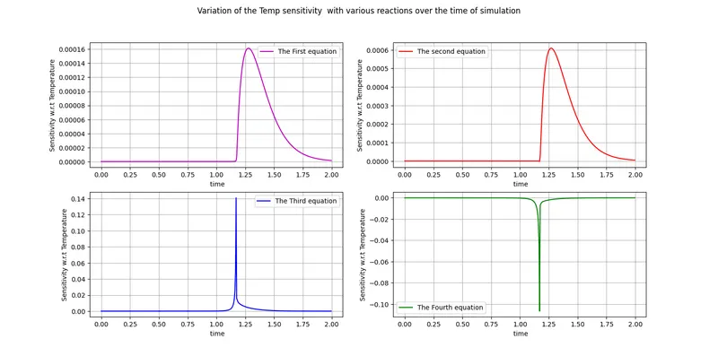
We can see that till autoignition temperature or the ignition delay time the sensitivity wrt all the reactions is almost zero sa the reactions are not happening in this zome.
Once the ignition delay time is attained, the temperature raises abruptly leading to the high sensitivity or gradient sa shown in the reactions