Week 5.1 - Mid term project - Solving the steady and unsteady 2D heat conduction problem
problem at hand:
1. Steady state analysis & Transient State Analysis
Solve the 2D heat conduction equation by using the point iterative techniques that were taught in the class. The Boundary conditions for the problem are as follows;
Top Boundary = 600 K
Bottom Boundary = 900 K
Left Boundary = 400 K
Right Boundary = 800 K
The Het conduction equation is given as: `(dt)/(dt) +alpha((d^2T)/(dx^2)+(d^2T)/(dy^2))=0`
Let us first begin by solving for the steady state solution which is:
`((d^2T)/(dx^2)+(d^2T)/(dy^2))=0`
The finite difference approximation used in this case is:
`T_p =(1/K)(((T_R +T_L)/(Deltax^2))+((T_T +T_B)/(Deltay^2)))`
The following iterative methods are used to solve the fintie difference approximations:
1. Jacobi
2. Gauss-seidel
3. Successive over-relaxation
the main file calls all the subroutines to evaluate the Temperature profile in the domain and them makes an subplot indicating the final solution from each iterative method. Along with the solution the time taken for each method with a fixed grid size of 100 by 100 nodes is shown.
For the small number of nodes the time of simulation may not vary much with all the methods but as the number of nodes increases the variation is eye catching.
The below is the code structure:
There are function files for each method
There is a boundary condition file, which is called in the each method function file and supplies the boundary conditions
one Main file to call all the routines
The code is as follows:
the Jacobi function file:
function [T] = jacobi(no_nodes_x, no_nodes_y,  delx , dely  , toleranace)

K=(2*(delx.^2+dely.^2))/((delx.^2)*(dely.^2)); % Declaring the constant variable which will be used further in the analysis:

%% Creating the Temperature Matrix to declare the boundary conditions
T=200*ones(no_nodes_x, no_nodes_y);  % declaring the temperature matrix of size of no.of nodes in x and no. of nodes in y

[T] = BC(T ); % calling the boundary conditions function file

jacobi_iteration=1;
error=99;
Told=T;

% toleranace=1e-04;

while (error>toleranace)

    for i=2:1:no_nodes_x-1 % looping over all the x nodes in the domain

        for j=2:1:no_nodes_y-1 % LOOPING OVER ALL the y nodes in the domain

             T(i,j)=((T(i-1,j)+T(i+1,j))./(K.*delx.^2))+((T(i, j-1)+T(i,j+1))./(K.*dely.^2));

        end  % end of the inner loop over all the y nodes

    end % end of for loop outermost

    error=max(max(abs(Told-T)));
    Told=T;
    jacobi_iteration =jacobi_iteration+1;
end


end
The gauss siedel function file:
function [T] = gauss_siedel(no_nodes_x, no_nodes_y,  delx , dely  , toleranace)

K=(2*(delx.^2+dely.^2))/((delx.^2)*(dely.^2)); % Declaring the constant variable which will be used further in the analysis:

%% Creating the Temperature Matrix to declare the boundary conditions
T=200*ones(no_nodes_x, no_nodes_y);  % declaring the temperature matrix of size of no.of nodes in x and no. of nodes in y

[T] = BC(T ); % calling the boundary conditions function file

gauss_siedel=1;
error=99;
Told=T;

% toleranace=1e-04;

while (error>toleranace)

    for i=2:1:no_nodes_x-1 % looping over all the x nodes in the domain

        for j=2:1:no_nodes_y-1 % LOOPING OVER ALL the y nodes in the domain

             T(i,j)=((T(i-1,j)+Told(i+1,j))./(K.*delx.^2))+((T(i, j-1)+Told(i,j+1))./(K.*dely.^2));

        end  % end of the inner loop over all the y nodes

    end % end of for loop outermost

    error=max(max(abs(Told-T)));
    Told=T;
    gauss_siedel =gauss_siedel+1;
end


end
the SOR function file:
function [T] = SOR(no_nodes_x, no_nodes_y,  delx , dely  , toleranace, omega)

K=(2*(delx.^2+dely.^2))/((delx.^2)*(dely.^2)); % Declaring the constant variable which will be used further in the analysis:

%% Creating the Temperature Matrix to declare the boundary conditions
T=200*ones(no_nodes_x, no_nodes_y);  % declaring the temperature matrix of size of no.of nodes in x and no. of nodes in y

[T] = BC(T ); % calling the boundary conditions function file

SOR_itr=1;
error=99;
Told=T;

% toleranace=1e-04;

while (error>toleranace)

    for i=2:1:no_nodes_x-1 % looping over all the x nodes in the domain

        for j=2:1:no_nodes_y-1 % LOOPING OVER ALL the y nodes in the domain

             T(i,j)=((1-omega)*Told(i,j))+omega*(((T(i-1,j)+Told(i+1,j))./(K.*delx.^2))+((T(i, j-1)+Told(i,j+1))./(K.*dely.^2)));

        end  % end of the inner loop over all the y nodes

    end % end of for loop outermost

    error=max(max(abs(Told-T)));
    Told=T;
    SOR_itr =SOR_itr+1;
end


end
The main file is:
%% This code is written by Noble Sharma to solve the 2d Heat equation on  3 Feb 2022 as a part of TSE -CFD Training
%% The challenge is  described in the Week  5.1
%%---------------------------------------------------------------------------------------------------------------------------------------------------------------------------------------
close all
clear all
clc

Length=1;  % Length of the domain
Width=1;    % Width  of the domain

no_nodes_x=100; % self declared no of nodes in x direction can be changed as user input also
no_nodes_y=100;% self declared no of nodes in y direction  can be changed as user input also

X_cord=linspace(0, Length, no_nodes_x); % Creating the locations on the Xaxis
Y_cord=linspace(Width, 0, no_nodes_y); % Creating the locations on the Yaxis

delx=Length/(no_nodes_x-1 );  % Calculating the distance between the grid points in the x direction
dely=Width/(no_nodes_y-1 );  % Calculating the distance between the grid points in the y direction


[XX,YY]=meshgrid( X_cord, Y_cord); % Creating the mesh grid to make an contor plot

tolerance=1e-04;
omega=1.2;

%% Function names created for the present work
% function [T] = gauss_siedel(no_nodes_x, no_nodes_y,  delx , dely  , tolerance)
%  function [T] = jacobi(no_nodes_x, no_nodes_y,  delx , dely  , tolerance)
% [T] = SOR(no_nodes_x, no_nodes_y,  delx , dely  , tolerance, omega)


tic
 [T1] = jacobi(no_nodes_x, no_nodes_y,  delx , dely  , tolerance);
 time(1)=toc;
tic
 [T2] =gauss_siedel(no_nodes_x, no_nodes_y,  delx , dely  , tolerance);
 time(2)=toc;
tic
 [T3] = SOR(no_nodes_x, no_nodes_y,  delx , dely  , tolerance, omega);
 time(3)=toc;


figure(1)
subplot(2,2,1)
[A, B]=contourf(XX,-YY,T1);
% [A, B]=contourf(XX,-YY,T)
% set(gca,'YDIR', 'reverse')
colormap(jet)
colorbar
clabel(A,B)
ylabel('Y');
xlabel('x');
title('iterative solving by Jacobi Method')

subplot(2,2,2)
[A, B]=contourf(XX,-YY,T2);
% [A, B]=contourf(XX,-YY,T)
% set(gca,'YDIR', 'reverse')
colormap(jet)
colorbar
clabel(A,B)
ylabel('Y');
xlabel('x');
title('iterative solving by Gauss siedel')


subplot(2,2,3)
[A, B]=contourf(XX,-YY,T3);
% [A, B]=contourf(XX,-YY,T)
% set(gca,'YDIR', 'reverse')
colormap(jet)
colorbar
clabel(A,B)
ylabel('Y');
xlabel('x');
title('iterative solving by SOR')

subplot(2,2,4)
A = categorical({'Jacobi','Gauss siedel','SOR'});
A = reordercats(A,{'Jacobi','Gauss siedel','SOR'});
bar(A, time, 0.5)
 xlabel('method used');
 ylabel('time taken');
title('relative performance of various iterative solvers')

%-------------------End of the code-----------------------%
The output obtained for the following input:
L=1;
W=1;
no_nodes_x=100;
no_nodes_y=100;
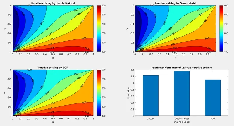
we can observe that all the iterative methods at the end converge to an solution which is quite the same, but the time taken by the solvers is not the same. SOR with an relaxation factor of 1.2 takes the lowest time comapared to other two.
Other thing which was observed that number of iterations taken by jacobi was the highest when compared to the gauss siedel or SOR.
Transient state analysis:
The transient solution is obtained from the below approximated solution:
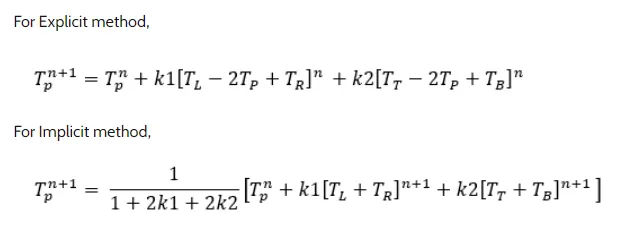
the below is the code for the explicit method:
%% This code is written by Noble Sharma to solve the 2d Heat equation on  3 Feb 2022 as a part of TSE -CFD Training
%% The challenge is  described in the Week  5.1
%%---------------------------------------------------------------------------------------------------------------------------------------------------------------------------------------
close all
clear all
clc
%% explicit method of solving the 2d unsteady heat  conduction

Length=1;  % Length of the domain
Width=1;    % Width  of the domain

no_nodes_x=100; % self declared no of nodes in x direction can be changed as user input also
no_nodes_y=100;% self declared no of nodes in y direction  can be changed as user input also
T=200*ones(no_nodes_x, no_nodes_y);  % declaring the temperature matrix of size of no.of nodes in x and no. of nodes in y
[T] = BC(T ); % calling the boundary conditions function file


X_cord=linspace(0, Length, no_nodes_x); % Creating the locations on the Xaxis
Y_cord=linspace(Width, 0, no_nodes_y); % Creating the locations on the Yaxis

delx=Length/(no_nodes_x-1 );  % Calculating the distance between the grid points in the x direction
dely=Width/(no_nodes_y-1 );  % Calculating the distance between the grid points in the y direction
[XX,YY]=meshgrid( X_cord, Y_cord); % Creating the mesh grid to make an contor plot

error=9;
tolerance=1e-04;
omega=1.2;

% declaring the time parameters
alpha=0.001;
delt=0.01;
time_steps=1400;
% declaring the CFL for X and Y directiopns
k1=(alpha*delt)/(delx^2);
k2=(alpha*delt)/(dely^2);

% Global CFL number
CFL_no=k1+k2 % declaring the CFL number for evalaution

Told=T;

iteration_count=1;

tic

for i =1:1:time_steps

    while (error>tolerance)

    for i=2:1:no_nodes_x-1 % looping over all the x nodes in the domain

        for j=2:1:no_nodes_y-1 % LOOPING OVER ALL the y nodes in the domain

             T(i,j)=Told(i,j)+k1*(Told(i-1,j)+Told(i+1,j)-2*Told(i, j))+k2*(Told(i, j-1)+Told(i,j+1)-2*Told(i,j));

        end  % end of the inner loop over all the y nodes

    end % end of for loop outermost

    error=max(max(abs(Told-T)));
    Told=T;
    iteration_count =iteration_count+1;
    end

end

 time=toc

  figure(1)
 [A, B]=contourf(XX,-YY,T);
% set(gca,'YDIR', 'reverse')
colormap(jet)
colorbar
clabel(A,B)
ylabel('Y');
xlabel('x');
title('Unsteady state solution  by explicit method')
Upon running the code we obtain the following solution:
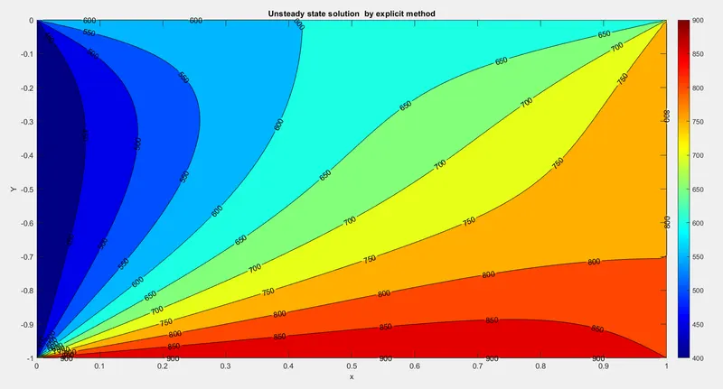
The temperature distribution satisfies the boundary conditions specified in the problem and also the contour lines indicate them. The CFL number used for the simulation was 0.1960 and the time taken by the simulation with the 100 by 100 node points is 8.9710 seconds.
since the bottom side is maintained at 900K the more heat is diffusing from the bottom and is shown in the coontour with the temperature shown inthe contour lines.
Implicit formulation:
Here again three methods used for the unsteady method are used and the modifications are made in the code to accomodate those in the function files. Additionally one main file is used to make the plots.
%% This code is written by Noble Sharma to solve the 2d Heat equation on  4 Feb 2022 as a part of TSE -CFD Training
%% The challenge is  described in the Week  5.1
%%---------------------------------------------------------------------------------------------------------------------------------------------------------------------------------------
close all
clear all
clc
%% Implicit  method of solving the 2d unsteady heat  conduction

Length=1;  % Length of the domain
Width=1;    % Width  of the domain

no_nodes_x=50; % self declared no of nodes in x direction can be changed as user input also
no_nodes_y=50;% self declared no of nodes in y direction  can be changed as user input also


X_cord=linspace(0, Length, no_nodes_x); % Creating the locations on the Xaxis
Y_cord=linspace(Width, 0, no_nodes_y); % Creating the locations on the Yaxis

delx=Length/(no_nodes_x-1 );  % Calculating the distance between the grid points in the x direction
dely=Width /(no_nodes_y- 1 );  % Calculating the distance between the grid points in the y direction

[XX,YY]=meshgrid( X_cord, Y_cord); % Creating the mesh grid to make an contor plot

tolerance=1e-04;
omega=1.2;

% declaring the time parameters
alpha=1.4;
delt=0.001;
time_steps=500;

T=298*ones(no_nodes_x, no_nodes_y);  % declaring the temperature matrix of size of no.of nodes in x and no. of nodes in y
[T] = BC(T ); % calling the boundary conditions function file

% declaring the CFL for X and Y directiopns
k1=(alpha*delt)/(delx^2);
k2=(alpha*delt)/(dely^2);

% Global CFL number
CFL_no=k1+k2; % declaring the CFL number for evalaution

% function [T,Gauss_siedel_iteration] =tran_Gauss_siedel(no_nodes_x, no_nodes_y,  toleranace, k1, k2, time_steps, T)

 tic
[T1, jacobi_iteration] =tran_jacob(no_nodes_x, no_nodes_y,  tolerance, k1, k2, time_steps, T);
time(1)=toc;

 tic
[T2, Gauss_siedel_iteration] =tran_Gauss_siedel(no_nodes_x, no_nodes_y,  tolerance, k1, k2, time_steps, T, XX,YY);
time(2)=toc;

 tic
[T3, SOR_iteration] =tran_SOR(no_nodes_x, no_nodes_y,  tolerance, k1, k2, time_steps, T, omega);
time(3)=toc;


figure(1)
subplot(2,2,1)
[A, B]=contourf(XX,-YY,T1);
% [A, B]=contourf(XX,-YY,T)
% set(gca,'YDIR', 'reverse')
colormap(jet)
colorbar
clabel(A,B)
ylabel('Y');
xlabel('x');
text=sprintf('Jacobi Method  and  Iterations = %d',jacobi_iteration);
title(text)


subplot(2,2,2)
[A, B]=contourf(XX,-YY,T2);
% [A, B]=contourf(XX,-YY,T)
% set(gca,'YDIR', 'reverse')
colormap(jet)
colorbar
clabel(A,B)
ylabel('Y');
xlabel('x');
text=sprintf('Gauss siedel Method and   Iterations = %d',Gauss_siedel_iteration);
title(text)

subplot(2,2,3)
[A, B]=contourf(XX,-YY,T3);
% [A, B]=contourf(XX,-YY,T)
% set(gca,'YDIR', 'reverse')
colormap(jet)
colorbar
clabel(A,B)
ylabel('Y');
xlabel('x');
text=sprintf('SOR  and Implicit Iterations = %d',SOR_iteration);
title(text)

subplot(2,2,4)
A = categorical({'Jacobi','Gauss siedel','SOR'});
A = reordercats(A,{'Jacobi','Gauss siedel','SOR'});
bar(A, time, 0.5)
 xlabel('method used');
 ylabel('time taken');
title('relative performance of various iterative solvers')

 %%---------------End of the Main file--------%
The function files are given below:
Jacobian Method:
function [T,jacobi_iteration] =tran_jacob(no_nodes_x, no_nodes_y,  toleranace, k1, k2, time_steps, T)

%% Creating the Temperature Matrix to declare the boundary conditions

jacobi_iteration=1;

Told=T;
T_prev_dt=T;
 % toleranace=1e-04;
ct=1;
for nt=1:time_steps
      term1=(1+2*k1+2*k2)^(-1);
      term2=k1*term1;
      term3=k2*term1;
       error=9e9;

 while(error>toleranace)
     for i=2:no_nodes_x-1
         for j=2:no_nodes_y-1
             a1=(Told(i-1,j)+Told(i+1,j));
             a2=(Told(i,j-1)+Told(i,j+1));
             T(i,j) = (T_prev_dt(i,j)*term1)+(a1*term2)+(a2*term3);
         end
     end

 error=max(max(abs(Told-T)));
 Told=T;
 jacobi_iteration=jacobi_iteration+1;
 end
  T_prev_dt=T;
%     figure(1)
% contourf(XX,YY,T)
% clabel(contourf(XX,YY,T))
% colorbar
% colormap(jet)
% set(gca,'ydir','reverse')
% xlabel('X -Axis')
% ylabel('Y -Axis')
% % pause(0.00000000000000003)
% M(ct)=getframe(gcf);
%  ct=ct+1;

 end %% end of function file
%  figure(55)
% movie(M)
% videofile=VideoWriter('jacobian.avi','Uncompressed Avi');
% open(videofile)
% writeVideo(videofile,M)
% close(videofile)

end
The function file for Gauss siedel:
function [T,Gauss_siedel_iteration] =tran_Gauss_siedel(no_nodes_x, no_nodes_y,  toleranace, k1, k2, time_steps, T, XX, YY)

%% Creating the Temperature Matrix to declare the boundary conditions
Gauss_siedel_iteration=1;
 Told=T;
T_prev_dt=T;
 % toleranace=1e-04;
ct=1;
for nt=1:time_steps
      term1=(1+2*k1+2*k2)^(-1);
      term2=k1*term1;
      term3=k2*term1;
       error=9e9;

 while(error>toleranace)
     for i=2:no_nodes_x-1
         for j=2:no_nodes_y-1
             a1=(T(i-1,j)+Told(i+1,j));
             a2=(T(i,j-1)+Told(i,j+1));
             T(i,j) = (T_prev_dt(i,j)*term1)+(a1*term2)+(a2*term3);
         end
     end

 error=max(max(abs(Told-T)));
 Told=T;
 Gauss_siedel_iteration=Gauss_siedel_iteration+1;
 end
  T_prev_dt=T;

%   figure(101)
% contourf(XX,YY,T)
% clabel(contourf(XX,YY,T))
% colorbar
% colormap(jet)
% set(gca,'ydir','reverse')
% xlabel('X -Axis')
% ylabel('Y -Axis')
% % pause(0.00000000000000003)
% M(ct)=getframe(gcf);
%  ct=ct+1;
end
%  figure(44)
% movie(M)
% videofile=VideoWriter('Gauss.avi','Uncompressed Avi');
% open(videofile)
% writeVideo(videofile,M)
% close(videofile)
%
end
The function file for SOR:
function [T,SOR_iteration] =tran_SOR(no_nodes_x, no_nodes_y,  toleranace, k1, k2, time_steps, T, omega)

%% Creating the Temperature Matrix to declare the boundary conditions
SOR_iteration=1;
Told=T;
T_prev_dt=T;
 % toleranace=1e-04;
ct=1;
for nt=1:time_steps
      term1=(1+2*k1+2*k2)^(-1);
      term2=k1*term1;
      term3=k2*term1;
       error=9e9;

 while(error>toleranace)
     for i=2:no_nodes_x-1
         for j=2:no_nodes_y-1
             a1=(T(i-1,j)+Told(i+1,j));
             a2=(T(i,j-1)+Told(i,j+1));
             T(i, j) =((1-omega)*Told(i, j))+ omega*((T_prev_dt(i ,j)*term1)+(a1*term2)+(a2*term3));
         end
     end

 error=max(max(abs(Told-T)));
 Told=T;
 SOR_iteration=SOR_iteration+1;
 end
  T_prev_dt=T;

 end %% end of function file

% figure(22)
% movie(M)
% videofile=VideoWriter('Gauss.avi','Uncompressed Avi');
% open(videofile)
% writeVideo(videofile,M)
% close(videofile)

end
The output is shown below:
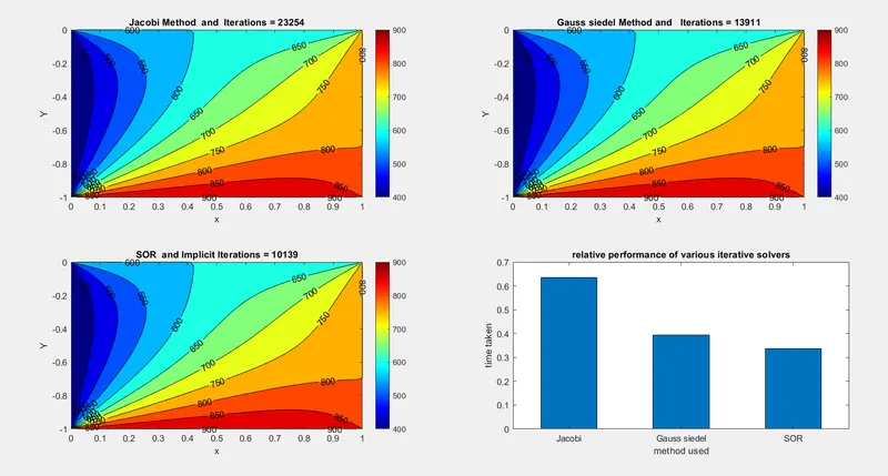
AS observed from the figure : the time taken for the SOR was the minimum when comared to other two methods.
The final contour is similar to the steady state solution. As per the information given in the
Ref: blog: https://skill-lync.com/knowledgebase/courant-number
The implicit schemes are far more stable and also unconditionally stable compared to the explicit schemes which required the CFL number to be less than half for the solution to be stable.