Week 3.5 - Deriving 4th order approximation of a 2nd order derivative using Taylor Table method
Derive the following 4th order approximations of the second-order derivative.
1. Central difference
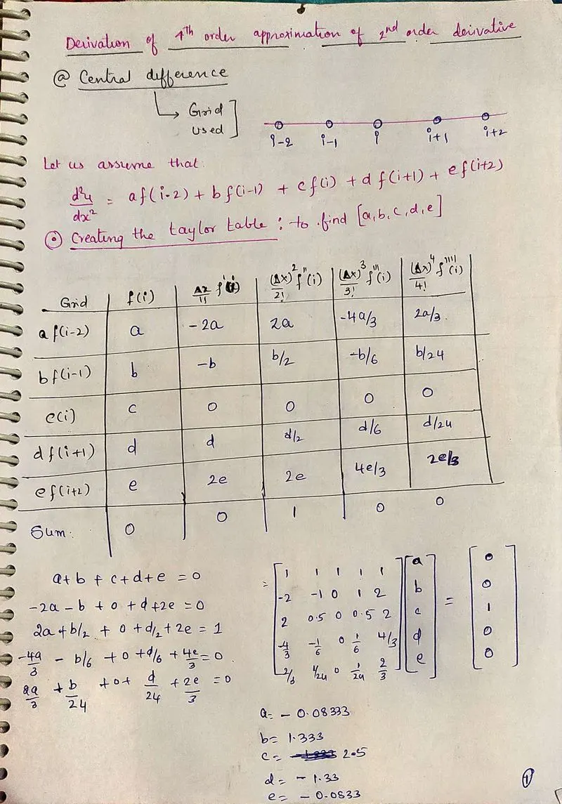
2. Skewed right-sided difference
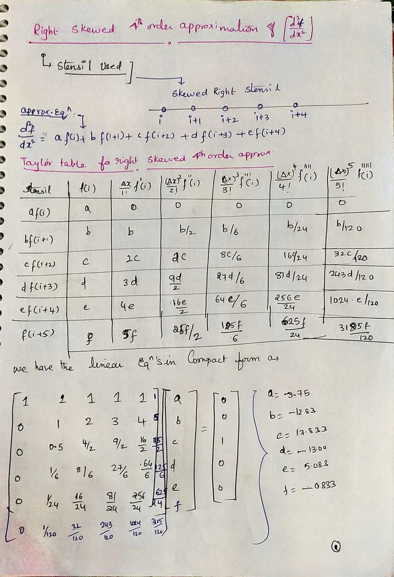
3. Skewed left-sided difference
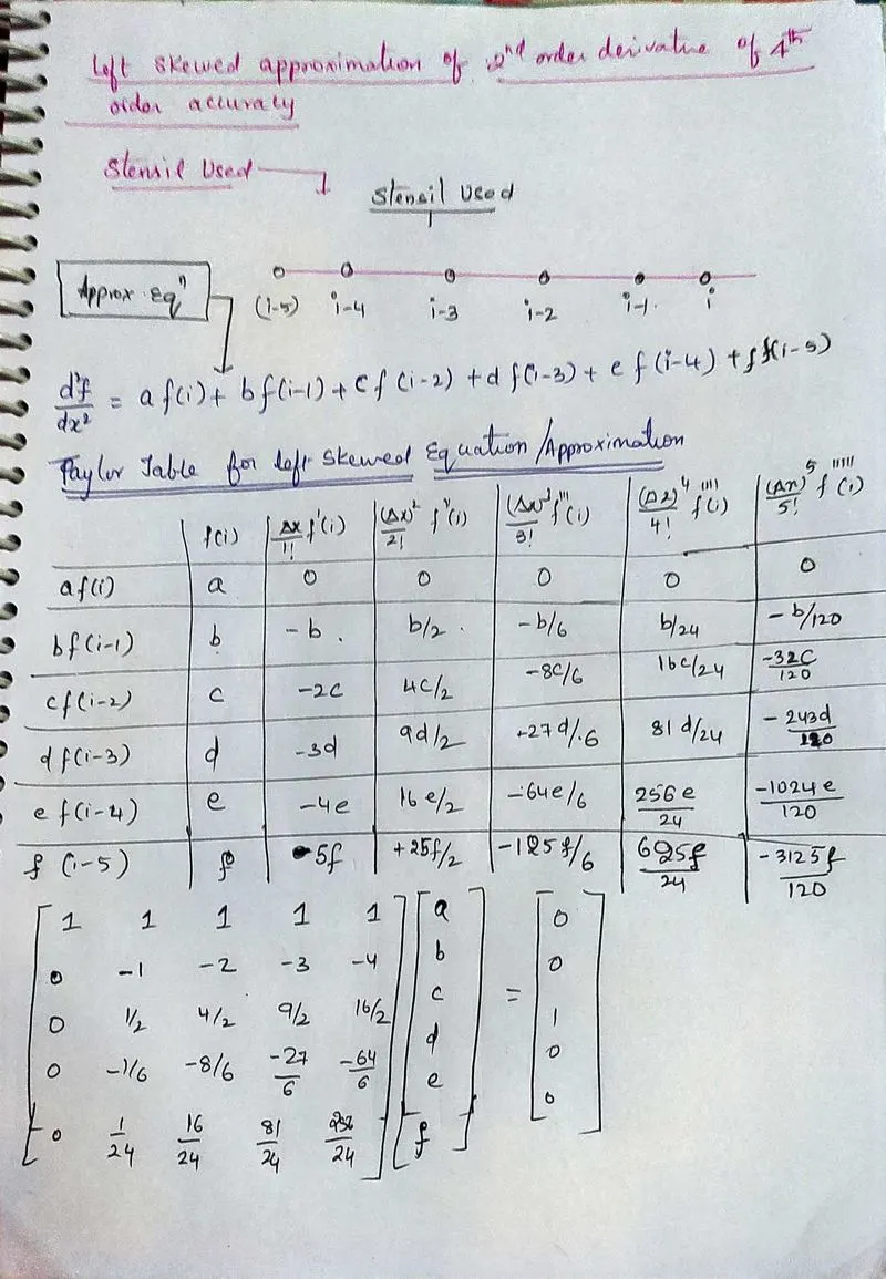
Verification of the accuracy being developed:
HINT :
i) The order of accuracy P = Number of nodes in the stencil N - order of derivative Q + 1 for symmetric/central schemes
For the central difference scheme: order of accuracyp=5-2+1=4 order accuracy
ii) The order of accuracy P = Number of nodes in the stencil N - order of derivative Q for one-sided/skewed schemes
For the right/ left skewed difference scheme: order of accuracy p =5-2=3 order accuracy
%% This code is written by Noble Sharma to demonstrate the use of taylor table to solve 4 order approximation  on 2 Feb 2022 as a part of TSE -CFD Training
%% The challenge is  described in the Week  3.5
%%---------------------------------------------------------------------------------------------------------------------------------------------------------------------------------------
close all
clear all
clc
%% the analytical function given at hand is exp(x)cos(x)
%%The analytical 2nd order derivative: exp(x)cos(x)-exp(x)sin(x)
x=pi/3; % the value of the x where the derivative is to be evaluated
Analytical_derivative= -2*exp(x)*sin(x);

%% Working on the evaluation by approximate methods
dx = linspace(pi/3,pi/3000,20);
% dx=pi/200
%% Evaluating the coefficients for the central differnce scheme of 4 order accuracy
%d^2(f)/dx^2=af(i-2)+bf(i-1)+cf(i)+df(i+1)+ef(i+2)
a1 = [1 1 1 1 1 ; -2 -1 0 1 2 ; 2 0.5 0 0.5 2 ; -4/3 -1/6 0 1/6 4/3 ; 2/3 1/24 0 1/24 2/3];
b1 = [0 ; 0 ; 1 ; 0 ; 0];
c1 = linsolve(a1,b1);  % c1=[a,b,c,d,e] of the central differnce method

%% Evaluating the coefficients for the right skewed  scheme of 4 order accuracy
%d^2(f)/dx^2=af(i)+bf(i+1)+cf(i+2)++df(i+3)+ef(i+4)++ff(i+5)
% A total of 6 nodes in the stenscil are required here as per the
% standandard norm specified in the prooblem
a2=[1  1 1 1 1 1 ; 0 1 2 3 4 5 ; 0, 1/2,  4/2,  9/2, 16/2, 25/2; 0, 1/6, 8/6, 27/6, 64/6, 125/6; 0, 1/24, 16/24, 81/24, 256/24, 625/24;  0, 1/120, 32/120, 243/120, 1024/120, 3125/120];
b2=[0 ;0;1;0;0;0];
c2= linsolve(a2,b2);

%% Evaluating the coefficients for the Left skewed  scheme of 4 order accuracy
%d^2(f)/dx^2=af(i)+bf(i-1)+cf(i-2)++df(i-3)+ef(i-4)++ff(i-5)
% A total of 6 nodes in the stenscil are required here as per the
% standandard norm specified in the prooblem
a3=[1  1 1 1 1 1 ; 0 -1 -2 -3 -4 -5 ; 0, 1/2,  4/2,  9/2, 16/2, 25/2; 0, -1/6, -8/6, -27/6, -64/6, -125/6; 0, 1/24, 16/24, 81/24, 256/24, 625/24;  0, -1/120, -32/120, -243/120, -1024/120, -3125/120];
b3=[0 ;0;1;0;0;0];
c3= linsolve(a3,b3);

for i = 1 : 1: length(dx)
        % %central_differencing
        Derivative_central_differencing(i) = ((c1(1)*exp(x-(2*dx(i)))*cos(x-(2*dx(i))))+(c1(2)*exp(x-dx(i))*cos(x-dx(i)))+ (c1(3)*exp(x)*cos(x))+(c1(4)*exp(x+dx(i))*cos(x+dx(i)))+(c1(5)*exp(x+(2*dx(i)))*cos(x+(2*dx(i)))))/(dx(i)^2);

        % % Skewed_right_sided_difference
        Derivative_Skewed_right_side(i) = ((c2(1)*exp(x)*cos(x))+(c2(2)*exp(x+dx(i))*cos(x+dx(i)))+(c2(3)*exp(x+ (2*dx(i)))*cos(x+(2*dx(i))))+(c2(4)*exp(x+(3*dx(i)))*cos(x+(3*dx(i))))+(c2(5)*exp(x+(4*dx(i)))*cos(x+(4*dx(i))))+(c2(6)*exp(x+ (5*dx(i)))*cos(x+(5*dx(i)))))/(dx(i)^2);

        % % Skewed_left_sided_difference
        Derivative_Skewed_left_side(i) = ((c3(1)*exp(x)*cos(x))+(c3(2)*exp(x-dx(i))*cos(x-dx(i)))+(c3(3)*exp(x- (2*dx(i)))*cos(x-(2*dx(i))))+(c3(4)*exp(x-(3*dx(i)))*cos(x-(3*dx(i))))+(c3(5)*exp(x-(4*dx(i)))*cos(x-(4*dx(i))))+ (c3(6)*exp(x-(5*dx(i)))*cos(x-(5*dx(i)))))/(dx(i)^2);

        % % % Error Calculation
        central_differencing_error(i) = abs(Derivative_central_differencing(i)-Analytical_derivative);
        Skewed_right_sided_difference_error(i) = abs(Derivative_Skewed_right_side(i)-Analytical_derivative);
        Skewed_left_sided_difference_error(i) = abs(Derivative_Skewed_left_side(i)-Analytical_derivative);
end


%% Plotting the  plot using the command bar(X,Y)
figure(1)
plot(dx, central_differencing_error, '-ro')
hold on
plot(dx, Skewed_right_sided_difference_error, '-bs')
hold on
plot(dx, Skewed_left_sided_difference_error, '-m^')
xlabel('range of Delta x')
ylabel(' Approximated values with various schemes')
legend('central differencing error', 'Skewed right sided difference error' , 'Skewed left sided difference error', 'FontSize',12,'FontWeight','bold')
grid on
hold off
%% Plotting the logarithemic curve for the visulaization of the lines as the absolute error variation is not appriciable from the above plot

figure(2)
loglog(dx, central_differencing_error, '-ro')
hold on
loglog(dx, Skewed_right_sided_difference_error, '-bs')
hold on
loglog(dx, Skewed_left_sided_difference_error, '-m^')
xlabel('range of Delta x')
ylabel(' Approximated values with various schemes')
legend('central differencing error', 'Skewed right sided difference error' , 'Skewed left sided difference error', 'FontSize',12,'FontWeight','bold')
grid on
hold off
%% Another way to visualize the differnece in the errors is to normalize the errors in the range of 0 to 1 and  that is what is done in the code below"
figure(3)
plot(dx, central_differencing_error./(max(central_differencing_error)), '-ro')
hold on
plot(dx, Skewed_right_sided_difference_error./(max(Skewed_right_sided_difference_error)), '-bs')
hold on
plot(dx, Skewed_left_sided_difference_error./(max(Skewed_left_sided_difference_error)), '-m^')
xlabel('range of Delta x')
ylabel(' Approximated values with various schemes with Normalization')
legend('Normalized central differencing error', 'Normalized Skewed right sided difference error' , 'Normalized Skewed left sided difference error', 'FontSize',12,'FontWeight','bold')
grid on
hold off
%%----------------------------------End of the code-----------------------
Upon running the code we obtain the following error plot:
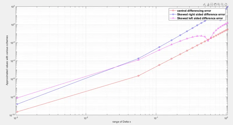
From the figure it can be seen that the error is minimum in the central difference scheme. If we want to compare the left and right skewed schemes then for a bigger grid size the left skewed scheme is more efficient, but as we reduce the grid size it is observed that the right skewed shceme performs better in terms of error reduction.
In order to show the big difference in the error's occuring at the differnce schemes used, i have made a plot between dx v/s actual error as shown below:
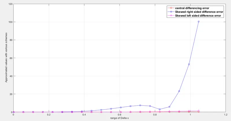
we can observe that the error is kinda very high in case of an right skewed scheme compared to others and central differnece has the least error.
In your own words, describe why a skewed scheme is useful? What can a skewed scheme do that a CD scheme cannot?
In a case where there are nodes only in the right or left, using central differce scheme we cannot evaluate the derivative.
if there is only one node on the left and five nodes on the right and we are required to fourth order approx. Only skewed schemes function well for a second derivative at that moment..if we want to compute a single or higher-order derivative a corner node then the central scheme is no longer useful.