Week 7 - Simulation of a 1D Super-sonic nozzle flow simulation using Macormack Method

Problem at Hand:

In this challenge you are going to simulate the isentropic flow through a quasi 1D subsonic-supersonic nozzle. You will derive both the conservation and non-conservation forms of the governing equations and sovle them using the MacCormack's technique. You need to determine the steady-state temperature distribution for the flow-field variables and investigate the difference between the two forms of governing equations by comparing their solutions.

You need to show the following plots inside your report
1. Steady-state distribution of primitive variables inside the nozzle
2. Time-wise variation of the primitive variables
3. Variation of Mass flow rate distribution inside the nozzle at different time steps during the time-marching process
4. Comparison of Normalized mass flow rate distributions of both forms

Solution:

Assumptions: Isentropic flow through Nozzle.

The Simulation is carried out by using finite differnece metnods utilizing the Macmormack's technique. This technique is second order accurate, Fully explicit by nature and quite straight forward to implement.

Steps involved:

• Deriving Governing equations:
• Discretizing the domain of interest
• Applying the Macormack's technique to solve equations
• Making the plots for visualization

Deriving Governing equations:

There are two kinds of forms of equations we can work on with

1. conservative form
2. Non conservative

Both of which are programmed to see the relative differences. The governing equations are:

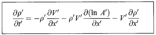
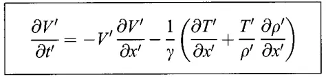
Non conservative: All the equations are referred from anderson text book and equations are written in non dimensional form

Continuity Equation

Momentum Equation

Energy Equation

conservative form:

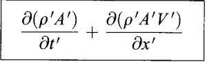
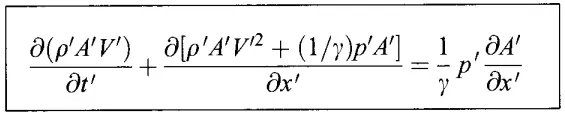
All the equation presented here are referred from the anderson text book and all the equations are written in the non dimensional form to ease the programming difficulties

continuity Equation:

Momentum Equation

Energy Equation:

Let us define three variables to make the equations look in more generic form which can be easily programmed:

• Solution vector U
• Source term J
• Flux term F

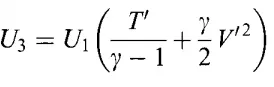
The genric form of the equations without primitive variables is given below:

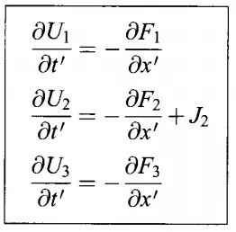
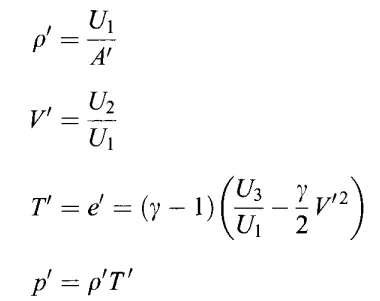
Writing the Flux terms also in terms of solution vector( this is needed since writing F in terms of primitives leads to instability)

• 
• 
• 
• 

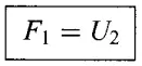
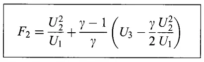
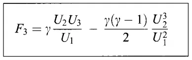
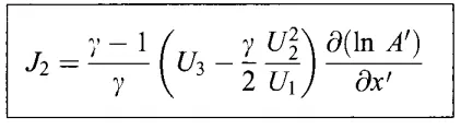
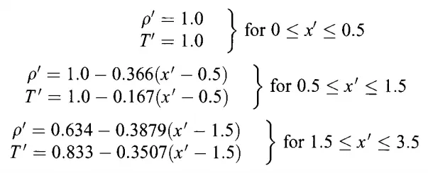
The inital conditions are calculated as follows:

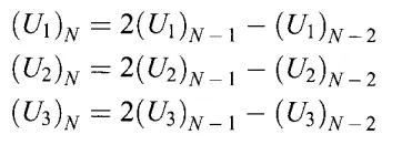
Boundary conditions:

at Nth node :

at 1st node :

Discretizing the domain of interest

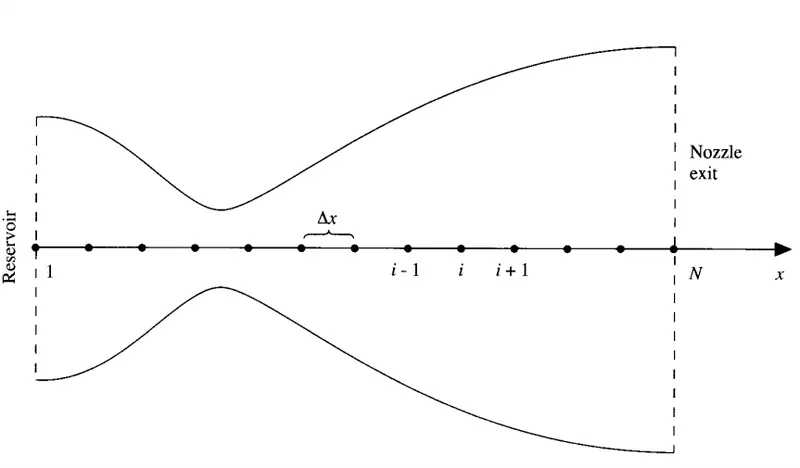
Domain is discretized to N nodes with 1 node indicating the reservoir where the inflow boundary conditions is specified and the node N is used for the outflow boundary conditions.

Applying the Macormack's technique to solve equations

Its a two step procedure:

• predictor step
• corrector step

Predictor step

Continuity Equation: replace all the spatial derivatives with forward differences:

Momentum Equation: replace all the spatial derivatives with forward differences:

Energy Equation: replace all the spatial derivatives with forward differences:

The predicted values of the primitive variables using taylor series expansion is:

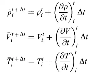
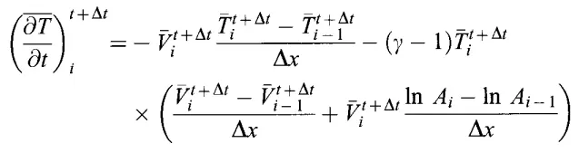
Corrector step: replace all the spatial derivatives with Backward differences:

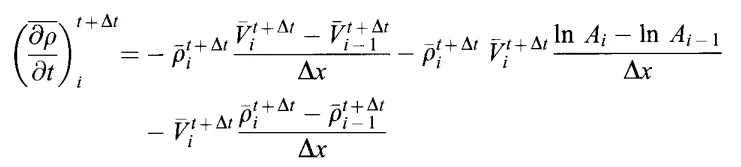
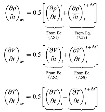
Finding the average value of derivative : This term is actually providing us the second order accuracy

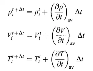
The final update of the primitive variable using the taylor series expansion and the avaraged derivative shown above is :

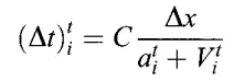
Time step calculation:

Two ways it can be done

• min of all the time steps at all the nodes
• local time stepping at each node

we are going with the method o1 as it maintains the global time stepping method and it will be easy to interpret resuts in the same time scale every where.

Boundary conditions:

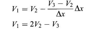
@node 01: subsonic flow:

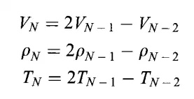
@node N: supersonic flow:

Geometry features

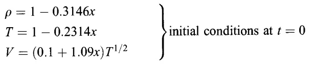
Initial Conditions:

The file structure used for solving and visulaizing the data is as follows:

• Main run file
• Function file to solve conservative equations
• Function file to solve Non conservative equations
• Function file to plot the results of conservative equations
• Function file to plot the results of Non conservative equations

Function file to solve the non condervative form of equations:

function [steady_state_sol, Variables_throat,Variables_location_transient, Variables1_location_transient,Avg_derivatives_location_transient ,Mass_flow_rate_initial ] = Non_conservative(no_nodes )
%% declaring the geometric parameters and other parameters of interest
L=3;  % Length of the nozzle
% no_divisions=90; % No. of divisions in the domain 
% no_nodes = no_divisions+1; % umber of Nodes in the domain
x_location = linspace(0,L,no_nodes); % Location of the nodes in the domain
Deltax=x_location(2)-x_location(1); % distance between the two nodes or delta x 
throat = (no_nodes+1)/2; % assuming equal no of grid points on either side of throat

No_time_steps = 1400; % Time of simulation 
CFL_no = 0.5; % Courant number and is less than unity
tol = 1e-4; % 
mdot_analytical = 0.579*ones(no_nodes);

%% Evaluating the area and Properties for the intial calculations
Area=1+2.2*(x_location-1.5).^2;
Density=1-0.3146.*x_location;
Temperature=1-0.2314.*x_location;
Velocity=(0.1+1.09.*x_location).*(Temperature.^(0.5));

 % copy of initial values
 Density_initial = Density;
 T_initial = Temperature;
 Vel_initial = Velocity;
  Mass_flow_rate_initial = Density.*Velocity.*Area;
 Mass_flow_rate_old = Density.*Velocity.*Area;

%   Delta_t= min((CFL_no.*Deltax)./(Temperature.^(1/2)+Velocity))
 
Gamma=1.4; % cp/cv
n_iter=1;
 error=1;
Time=0;

for i=1:1:No_time_steps
      
    % storing the values for the update
    Temperature_old=Temperature; %% Storing the Temperature
    Density_old=Density;   %% Storing the density
    Velocity_old=Velocity;%% Storing the Velocity
     
    %% determining the delta 't' for every iteration count
    Delta_t= min((CFL_no.*Deltax)./(Temperature.^(1/2)+Velocity));  %% evaluating the delta t for each time iteration
    delta_t(i,:)=Delta_t;
    
    Time=Time+Delta_t;
    dummy_time(i,:)=Time;
    
      for j=2:1:no_nodes-1

         %% Evalauting the derivatives which are frequently used and also to improvide the readability of the code
         Del_V_byDelx=(Velocity(j+1)-Velocity(j))./(Deltax);
         Del_rho_byDelx=(Density(j+1)-Density(j))./(Deltax);
         Del_logA_byDelx=(log(Area(j+1))-log(Area(j)))./(Deltax);
         Del_Temp_byDelx=(Temperature(j+1)-Temperature(j))./(Deltax);
         
        %% Evaluating the derivatives with the forward differences  (for predictor step)
         %% Continuity equation: Provides the: D(rho)/D(t)
         Del_rho_byDelt_pred(j)=(-Density(j).*Del_V_byDelx) - (Density(j).*Velocity(j).*Del_logA_byDelx) - (Velocity(j).*Del_rho_byDelx);
         %% Momentum Equation: Provides : D(Vel)/D(t)
         Del_V_byDelt_pred(j)=(-Velocity(j).* Del_V_byDelx)-(Gamma.^-1).*((Del_Temp_byDelx)+(Temperature(j).*(Density(j).^-1).*Del_rho_byDelx));
        %% Energy Equation: Provide : D(Temp)/D(t)
         Del_Temp_byDelt_pred(j)=-(Velocity(j).*Del_Temp_byDelx)-((Gamma-1).*Temperature(j).*(Del_V_byDelx+Velocity(j).*Del_logA_byDelx));
                  
        %% Predictor step Update of the primary variables uisng the Taylor series expansion 
        Density(j)=Density_old(j)+ Del_rho_byDelt_pred(j).*Delta_t;
        Temperature(j)=Temperature_old(j)+Del_Temp_byDelt_pred(j).*Delta_t;
        Velocity(j)=Velocity_old(j)+Del_V_byDelt_pred(j).*Delta_t;
         
       %%%%% %%    Corrector step Begins at this step   %%%%%%%%%%%%%%%
         %% Evalauting the derivatives for density temp, velocity with the values obtained in the end of the predictor step (backward differencing)
          Del_V_byDelx=(Velocity(j)-Velocity(j-1))./(Deltax);
         Del_rho_byDelx=(Density(j)-Density(j-1))./(Deltax);
         Del_logA_byDelx=(log(Area(j))-log(Area(j-1)))./(Deltax);
         Del_Temp_byDelx=(Temperature(j)-Temperature(j-1))./(Deltax);
         
         %% Evaluating the derivatives of the quantities using the corrector method 
         % Continuity equation: D(rho)/D(t)
          Del_rho_byDelt_Corr(j)=(-Density(j).*Del_V_byDelx) - (Density(j).*Velocity(j).*Del_logA_byDelx) - (Velocity(j).*Del_rho_byDelx);
          %% Momentum Equation: Provides : D(Vel)/D(t)       
          Del_V_byDelt_Corr(j)=(-Velocity(j).* Del_V_byDelx)-(Gamma.^-1).*((Del_Temp_byDelx)+(Temperature(j).*(Density(j).^-1).*Del_rho_byDelx));
        %% Energy Equation: Provide : D(Temp)/D(t)
          Del_Temp_byDelt_Corr(j)=-(Velocity(j).*Del_Temp_byDelx)-((Gamma-1).*Temperature(j).*(Del_V_byDelx+Velocity(j).*Del_logA_byDelx));
         
         %% Evaluating the average value of the derivatives for the update
         Del_rho_byDelt_Avg(j)=0.5.*(Del_rho_byDelt_Corr(j)+Del_rho_byDelt_pred(j));
         Del_rho_byDelt_Avg_dummy(i,j)=Del_rho_byDelt_Avg(j);
         
         Del_Temp_byDelt_Avg(j)=0.5.*(Del_Temp_byDelt_Corr(j)+Del_Temp_byDelt_pred(j));
         Del_Temp_byDelt_Avg_dummy(i,j)=Del_Temp_byDelt_Avg(j);
         
         Del_V_byDelt_Corr_Avg(j)=0.5.*(Del_V_byDelt_Corr(j)+Del_V_byDelt_pred(j));
         Del_V_byDelt_Corr_Avg_dummy(i,j)=  Del_V_byDelt_Corr_Avg(j) ;
           
         %% Corrector step update of the design variables using the averaged derivatives : Here also we will use the taylor series expansion as used 
         %% in the end step of the predictor step 
         Density(j)=Density_old(j)+ Del_rho_byDelt_Avg(j).*Delta_t;
         Density_dummy(i,j)=Density(j);
        Temperature(j)=Temperature_old(j)+Del_Temp_byDelt_Avg(j).*Delta_t;
        Temperature_dummy(i,j)=  Temperature(j);
        Velocity(j)=Velocity_old(j)+Del_V_byDelt_Corr_Avg(j).*Delta_t;
        Velocity_dummy(i,j)=Velocity_old(j);
         
      end 
    
    %%Updating the Boundary conditions i.e. the floater variables at the
    %%boundary nodes 

    %% Inlet boundary condition i.e. at the node 01
    Velocity(1) = 2*Velocity(2)-Velocity(3);
    % Outlet boundary conditions i.e. at node N
    Velocity(no_nodes) = 2*Velocity(no_nodes-1)-Velocity(no_nodes-2);
    Density(no_nodes) = 2*Density(no_nodes-1)-Density(no_nodes-2);
    Temperature(no_nodes) = 2*Temperature(no_nodes-1)-Temperature(no_nodes-2);
    
     % Calculating pressure, mass flow rate and Mach number
      Mach_num = Velocity./Temperature.^0.5;  % Mach number 
      Mach_num_dummy(i,:)=Mach_num; % Mach number storing for every node and iteration of time step
       Pressure=Density.*Temperature;
       Pressure_dummy(i,:)=Pressure;
      Mass_flow_rate(i, :)=Density.*Area.*Velocity;
       Mass_flow=Density.*Area.*Velocity;

    % Capturing flow field variables at the throat for each time step
    Density_throat(i) = Density(throat);
    Temperature_throat(i) = Temperature(throat);
    Pressure_throat(i) = Pressure(throat);
    Mach_num_throat(i) = Mach_num(throat);
    
    % checking convergence
    error = max(abs( Mass_flow-Mass_flow_rate_old));
    if error>tol
    n_iter = n_iter + 1; 
    Mass_flow_rate_old = Mass_flow;
    end
      
end 

%% Used to store the variables to reduce the count of matrices
Variables_throat(1,:)=Density_throat;
Variables_throat(2,:)=Temperature_throat;
Variables_throat(3,:)=Pressure_throat;
Variables_throat(4,:)=Mach_num_throat;

steady_state_sol(1,:)=Density;
steady_state_sol(2,:)=Temperature;
steady_state_sol(3,:)=Pressure;
steady_state_sol(4,:)=Mach_num;
steady_state_sol(5,:)=Mass_flow;


Variables_location_transient(:, :, 1)=Density_dummy;
Variables_location_transient(:, :, 2)=Temperature_dummy;

Variables1_location_transient(:, :, 1)=Pressure_dummy;
Variables1_location_transient(:, :, 2)=Mach_num_dummy;
Variables1_location_transient(:, :, 3)=Mass_flow_rate;

Avg_derivatives_location_transient(:,:,1)=Del_rho_byDelt_Avg_dummy;
Avg_derivatives_location_transient(:,:,2)=Del_V_byDelt_Corr_Avg_dummy;
Avg_derivatives_location_transient(:,:,3)=Del_Temp_byDelt_Avg_dummy;

end

The function file to solve the conservative form of equations is:

function [steady_state_sol, Variables_throat,Variables_location_transient, Variables1_location_transient,Avg_derivatives_location_transient,Mass_flow_rate_initial] = conservativeform(no_nodes)

%% declaring the geometric parameters and other parameters of interest
L=3;  % Length of the nozzle
% no_divisions=90; % No. of divisions in the domain 
% no_nodes = no_divisions+1; % umber of Nodes in the domain
x_location = linspace(0,L,no_nodes); % Location of the nodes in the domain
Deltax=x_location(2)-x_location(1); % distance between the two nodes or delta x 
throat = (no_nodes+1)/2; % assuming equal no of grid points on either side of throat

No_time_steps = 1400; % Time of simulation 
CFL_no = 0.5; % Courant number and is less than unity
tol = 1e-4; % 

%% mass flow rate analytical
mdot_analytical = 0.579*ones(no_nodes);
Gamma=1.4;
n_iter=1;
 error=1;
Time=0;

%% Evaluating the area and Properties for the intial calculations
Area=1+2.2*(x_location-1.5).^2;
u2_i = 0.59; % initial mass flow rate, at t=0;

for i=1:1:no_nodes
    
    if(x_location(i)>=0 && x_location(i)<=0.5)
        Density(i)=1;
        Temperature(i)=1;
        
    elseif (x_location(i)>0.5  && x_location(i)<1.5)
          Density(i)=1-0.366*(x_location(i)-0.5);
        Temperature(i)=1-0.167*(x_location(i)-0.5);
                
    elseif (x_location(i)>=1.5  && x_location(i)<=3)
           Density(i)= 0.634-0.3879*(x_location(i)-1.5);
        Temperature(i)= 0.833-0.3507*(x_location(i)-1.5);
        
    end 
 Velocity(i) = u2_i/(Density(i)*Area(i));
 U1(i) = Density(i)*Area(i);
 U2(i) = Density(i)*Area(i)*Velocity(i);
 U3(i) = Density(i)*Area(i)*(Temperature(i)./(Gamma-1)+(Gamma./2)*Velocity(i)^2);    
end 

 % copy of initial values
 Velocity_initial=Velocity;
  U1_initial = U1; % Storing the initial conditions 
 U2_initial = U2;
 U3_initial = U3;
 
 Mass_flow_rate_initial = Density.*Velocity.*Area;
 Mass_flow_rate_old = Density.*Velocity.*Area;

for i=1:1:No_time_steps
      
    % storing the values for the update
     U1_old = U1;
     U2_old = U2;
     U3_old = U3;
     
    %% determining the delta 't' for every iteration count
    Delta_t= min((CFL_no.*Deltax)./(Temperature.^(1/2)+Velocity));  %% evaluating the delta t for each time iteration
    delta_t(i,:)=Delta_t;
    
    Time=Time+Delta_t; % trial just to store the time 
    dummy_time(i,:)=Time;

   
     for j = 2:1:no_nodes-1
         
         %% Predictor step starts from here: %%%
        %% Evaluation of the flux terms     
         F1_i = U2(j);   % F at j node
         F1_iPlus1=U2(j+1);   % F atj+1 node
         
         F2_i=U2(j)^2/U1(j)+((Gamma-1)/Gamma)*(U3(j)-(Gamma/2)*U2(j).^2/U1(j)); % F2 at j node
         F2_iPlus1=U2(j+1)^2/U1(j+1)+((Gamma-1)/Gamma)*(U3(j+1)-(Gamma/2)*U2(j+1).^2/U1(j+1));% F2 atj+1 node
         
         F3_i = Gamma*U2(j)*U3(j)/U1(j)-(Gamma*(Gamma-1)/2)*U2(j)^3/U1(j)^2; % F3 at j node
         F3_iPlus1 = Gamma*U2(j+1)*U3(j+1)/U1(j+1)-(Gamma*(Gamma-1)/2)*U2(j+1)^3/U1(j+1)^2 ;% F3 atj+1 node
        
          j2 = (1/Gamma)*Density(j)*Temperature(j)*((Area(j+1) - Area(j))/Deltax);  % Source term 
         
                 %% Evaluating the derivatives with the forward differences  (for predictor step)
           Del_U1_byDelt_pred(j)=-(F1_iPlus1-F1_i)./Deltax; % 
           Del_U2_byDelt_pred(j)=(-(F2_iPlus1-F2_i)./Deltax) +j2;% DU2/Dt
           Del_U3_byDelt_pred(j)=-(F3_iPlus1-F3_i)./Deltax;% DU3/Dt
           
           %% Predictor step Update of the solution  variables uisng the Taylor series expansion 
         U1(j) = U1(j)+Del_U1_byDelt_pred(j)*Delta_t; %U1= U1+DU1/Dt*dt
         U2(j) = U2(j)+Del_U2_byDelt_pred(j)*Delta_t;%U2= U1+DU1/Dt*dt
         U3(j) = U3(j)+Del_U3_byDelt_pred(j)*Delta_t;%U3= U1+DU1/Dt*dt
         
         %EEvaluating the primitive variables 
         Density(j)= U1(j)./Area(j);
         Velocity(j)=U2(j)./U1(j);
         Temperature(j)= (Gamma-1)*((U3(j)./U1(j)) - (Gamma/2)*Velocity(j).^2);
         
       %%%%% %%    Corrector step Begins at this step   %%%%%%%%%%%%%%%
         %% Evalauting the derivatives for density temp, velocity with the values obtained in the end of the predictor step (backward differencing) 
          F1_i = U2(j);
          F1_iMinus1 = U2(j-1);  
          
          F2_i=U2(j)^2/U1(j)+((Gamma-1)/Gamma)*(U3(j)-(Gamma/2)*U2(j).^2/U1(j));
          F2_iMinus1=U2(j-1)^2/U1(j-1)+((Gamma-1)/Gamma)*(U3(j-1)-(Gamma/2)*U2(j-1).^2/U1(j-1));
         
         F3_i = Gamma*U2(j)*U3(j)/U1(j)-(Gamma*(Gamma-1)/2)*U2(j)^3/U1(j)^2;
         F3_iMinus1 = Gamma*U2(j-1)*U3(j-1)/U1(j-1)-(Gamma*(Gamma-1)/2)*U2(j-1)^3/U1(j-1)^2;
        
          j2 = (1/Gamma)*Density(j)*Temperature(j)*((Area(j) - Area(j-1))/Deltax);
         
          %% Evaluating the derivatives with the forward differences  (for predictor step)
           Del_U1_byDelt_Corr(j)=-( F1_i-F1_iMinus1)./Deltax;
           Del_U2_byDelt_Corr(j)=(-(F2_i-F2_iMinus1)./Deltax) +j2;
           Del_U3_byDelt_Corr(j)=-(F3_i-F3_iMinus1)./Deltax;
         
         %% Evaluating the average value of the derivatives for the update
         Del_U1_byDelt_Avg(j)=0.5.*(Del_U1_byDelt_Corr(j)+Del_U1_byDelt_pred(j));
         Del_U2_byDelt_Avg(j)=0.5.*(Del_U2_byDelt_Corr(j)+Del_U2_byDelt_pred(j));
         Del_U3_byDelt_Avg(j)=0.5.*(Del_U3_byDelt_Corr(j)+Del_U3_byDelt_pred(j));
                 
         %% Corrector step update of the design variables using the averaged derivatives : Here also we will use the taylor series expansion as used 
         %% in the end step of the predictor step 
         U1(j) = U1_old(j)+Del_U1_byDelt_Avg(j)*Delta_t;
         U2(j) = U2_old(j)+Del_U2_byDelt_Avg(j)*Delta_t;
         U3(j) = U3_old(j)+Del_U3_byDelt_Avg(j)*Delta_t;         
         
         %% Additional array to store the variabels for plot
         U1_dummy(i,j) = U1_old(j)+Del_U1_byDelt_Avg(j)*Delta_t;
         U2_dummy(i,j) = U2_old(j)+Del_U2_byDelt_Avg(j)*Delta_t;
         U3_dummy(i,j) = U3_old(j)+Del_U3_byDelt_Avg(j)*Delta_t;              
         
     end 
    
             % Aditionally declaring dummy vriables to store the derivatives for
        % plotting
         Del_U1_byDelt_Avg_Dummy(i,:)=Del_U1_byDelt_Avg;
         Del_U2_byDelt_Avg_Dummy(i,:)=Del_U2_byDelt_Avg;
         Del_U3_byDelt_Avg_Dummy(i,:)=Del_U3_byDelt_Avg;     
     
   
   %%Updating the Boundary conditions i.e. the floater variables at the
   %%boundary nodes  
    
      U1(1) = Density(1)*Area(1);
     U2(1) = 2*U2(2)-U2(3);
     Velocity(1) = U2(1)/(Density(1)*Area(1));
     U3(1) = U1(1)*(Temperature(1)/(Gamma-1)+(Gamma/2)*Velocity(1)^2);
     % outlet
     U1(no_nodes) = 2*U1(no_nodes-1)-U1(no_nodes-2);
     U2(no_nodes) = 2*U2(no_nodes-1)-U2(no_nodes-2);
     U3(no_nodes) = 2*U3(no_nodes-1)-U3(no_nodes-2);   

     % Calculating pressure, mass flow rate and Mach number
     % computing the values of the primitive variables
     for k= 1:1:no_nodes
     Density(k) = U1(k)/Area(k);
     Velocity(k) = U2(k)/U1(k);
     Temperature(k) = (Gamma-1)*(U3(k)/U1(k)-Gamma/2*Velocity(k)^2);
     end
    
     Density_dummy(i,:)=Density;
     Velocity_dummy(i,:)=Velocity;
     Temperature_dummy(i,:)=Temperature;
     
     
     
      % Calculating pressure, mass flow rate and Mach number
      Mach_num = Velocity./Temperature.^0.5;
      Mach_num_dummy(i,:)=Mach_num;
      
       Pressure=Density.*Temperature;
       Pressure_dummy(i,:)=Pressure;
      
       Mass_flow_rate(i, :)=Density.*Area.*Velocity;
       Mass_flow=Density.*Area.*Velocity;
    
     % Capturing flow field variables at the throat for each time step
    Density_throat(i) = Density(throat);
    Temperature_throat(i) = Temperature(throat);
    Pressure_throat(i) = Pressure(throat);
    Mach_num_throat(i) = Mach_num(throat);
    
    % checking convergence
    error = max(abs( Mass_flow-Mass_flow_rate_old));
    if error>tol
    n_iter = n_iter + 1; 
    Mass_flow_rate_old = Mass_flow;
    end
    
   
end

%% Used to reduce the matrix compliations
Variables_throat(1,:)=Density_throat;
Variables_throat(2,:)=Temperature_throat;
Variables_throat(3,:)=Pressure_throat;
Variables_throat(4,:)=Mach_num_throat;

steady_state_sol(1,:)=Density;
steady_state_sol(2,:)=Temperature;
steady_state_sol(3,:)=Pressure;
steady_state_sol(4,:)=Mach_num;
steady_state_sol(5,:)=Mass_flow;


Variables_location_transient(:, :, 1)=Density_dummy;
Variables_location_transient(:, :, 2)=Temperature_dummy;

Variables1_location_transient(:, :, 1)=Pressure_dummy;
Variables1_location_transient(:, :, 2)=Mach_num_dummy;
Variables1_location_transient(:, :, 3)=Mass_flow_rate;

Avg_derivatives_location_transient(:,:,1)=Del_U1_byDelt_Avg_Dummy;
Avg_derivatives_location_transient(:,:,2)=Del_U2_byDelt_Avg_Dummy;
Avg_derivatives_location_transient(:,:,3)=Del_U3_byDelt_Avg_Dummy;

end 

Code used for post processing:

function [ ] = Post_processing_C(fig_num ,L,  no_divisions,No_time_steps, steady_state_sol, Variables_throat,Variables_location_transient, Variables1_location_transient,Avg_derivatives_location_transient,Mass_flow_rate_initial)
 
no_nodes = no_divisions+1; % umber of Nodes in the domain
x_location = linspace(0,L,no_nodes); % Location of the nodes in the domain
throat = (no_nodes+1)/2; % assuming equal no of grid points on either side of throat
mdot_analytical = 0.579*ones(no_nodes);

 figure(fig_num);
 sgtitle(sprintf(['Steady-state distribution of flow-field variables across nozzle'...
 '\n conservation form, No. of time steps = %g'],No_time_steps));
subplot(4,1,1)
 plot(x_location./L,steady_state_sol(4,:),'LineWidth',2);
 xlabel('x/L');
 ylabel('M');
 title(sprintf('Mach number'));
 grid on 
 
 subplot(4,1,2);
 plot(x_location./L,steady_state_sol(1,:),'r','LineWidth',2);
 xlabel('x/L');
 ylabel('\rho/\rho_o');
 title(sprintf('Non-dimensional Density'));
  grid on 

 subplot(4,1,3);
 plot(x_location./L,steady_state_sol(2,:),'g','LineWidth',2);
 xlabel('x/L');
 ylabel('T/T_o');
 title(sprintf('Non-dimensional Temperature'));
  grid on 

 subplot(4,1,4);
 plot(x_location./L,steady_state_sol(3,:),'m','LineWidth',2);
 xlabel('x/L');
 ylabel('p/p_o');
 title(sprintf('Non-dimensional Pressure'));
 grid on 

% Timewise variarion of flow field variables at nozzle throat
 figure(fig_num+1)
 plot( 1:No_time_steps,Variables_throat(1,:),'LineWidth',2);
 hold on
 plot(1:No_time_steps,Variables_throat(2,:),'LineWidth',2);
 hold on
 plot(1:No_time_steps,Variables_throat(3,:),'LineWidth',2);
 hold on
 plot(1:No_time_steps,Variables_throat(4,:),'LineWidth',2);
 title(sprintf(['Timewise variation of non-dimensional flow-field variables' '\nat nozzle throat- conservation form']));
 xlabel('Number of time steps');
 legend('\rho/\rho_o','T/T_o','p/p_o','M');
grid on 


figure(fig_num+2)
plot(x_location./L,Mass_flow_rate_initial,x_location./L,Variables1_location_transient(50, :, 3) ,x_location./L, Variables1_location_transient(100, :, 3),x_location./L,Variables1_location_transient(150, :, 3),...
 x_location./L,Variables1_location_transient(200, :, 3),x_location./L,Variables1_location_transient(700, :, 3),x_location./L,mdot_analytical,':','LineWidth',2);
 xlabel('Non-dimensional distance through nozzle(x)');
 ylabel('Non-dimensional mass flow (\rhoVA)/(\rho_oa_oA*)');
 legend('0\Deltat','50\Deltat','100\Deltat','150\Deltat','200\Deltat','700\Deltat','Analytical solution');
 title(sprintf(['Distribution of non-dimensional mass flow rate across the nozzle'...
 '\n-conservation form']));
grid on 

figure(fig_num+3)
subplot(4,1,1)
plot(1:No_time_steps,  Variables_location_transient(:, throat, 1), '-r','LineWidth', 2)
xlabel('number of time steps')
ylabel('( {\rho}/{ \rho_{0}})')
title(sprintf(['Time wise variation of density at nozzle throat where A=1']));
grid on

subplot(4,1,2)
plot(1:No_time_steps, Variables_location_transient(:, throat, 2), '-b','LineWidth', 2)
xlabel('number of time steps')
ylabel('( {T}/{ T_{0}})')
title(sprintf(['Time wise variation of Temperature at nozzle throat where A=1']));
grid on


subplot(4,1,3)
plot(1:No_time_steps, Variables1_location_transient(:, throat, 1) , '-m','LineWidth', 2)
xlabel('number of time steps')
ylabel('( {P}/{ P_{0}})')
title(sprintf(['Time wise variation of Pressure at nozzle throat where A=1']));
grid on

subplot(4,1,4)
plot(1:No_time_steps, Variables1_location_transient(:, throat, 2) , '-m','LineWidth', 2)
xlabel('number of time steps')
ylabel('M')
title(sprintf(['Time wise variation of Mach No at nozzle throat where A=1']));
grid on


figure(fig_num+4)
plot(1:No_time_steps, abs(Avg_derivatives_location_transient(:, throat, 1)) , '-m','LineWidth', 2)
hold on
plot(1:No_time_steps, abs(Avg_derivatives_location_transient(:, throat, 2)) , '-r','LineWidth', 2)
grid on

end

function [ ] = Post_processing_N(fig_num ,L,  no_divisions,No_time_steps, steady_state_sol, Variables_throat,Variables_location_transient, Variables1_location_transient,Avg_derivatives_location_transient,Mass_flow_rate_initial)
 
no_nodes = no_divisions+1; % umber of Nodes in the domain
x_location = linspace(0,L,no_nodes); % Location of the nodes in the domain
throat = (no_nodes+1)/2; % assuming equal no of grid points on either side of throat
mdot_analytical = 0.579*ones(no_nodes);

 figure(fig_num);
 sgtitle(sprintf(['Steady-state distribution of flow-field variables across nozzle'...
 '\n-Non-conservation form, No. of time steps = %g'],No_time_steps));
subplot(4,1,1)
 plot(x_location./L,steady_state_sol(4,:),'LineWidth',2);
 xlabel('x/L');
 ylabel('M');
 title(sprintf('Mach number'));
 grid on 
 
 subplot(4,1,2);
 plot(x_location./L,steady_state_sol(1,:),'r','LineWidth',2);
 xlabel('x/L');
 ylabel('\rho/\rho_o');
 title(sprintf('Non-dimensional Density'));
  grid on 

 subplot(4,1,3);
 plot(x_location./L,steady_state_sol(2,:),'g','LineWidth',2);
 xlabel('x/L');
 ylabel('T/T_o');
 title(sprintf('Non-dimensional Temperature'));
  grid on 

 subplot(4,1,4);
 plot(x_location./L,steady_state_sol(3,:),'m','LineWidth',2);
 xlabel('x/L');
 ylabel('p/p_o');
 title(sprintf('Non-dimensional Pressure'));
 grid on 

% Timewise variarion of flow field variables at nozzle throat
 figure(fig_num+1)
 plot( 1:No_time_steps,Variables_throat(1,:),'LineWidth',2);
 hold on
 plot(1:No_time_steps,Variables_throat(2,:),'LineWidth',2);
 hold on
 plot(1:No_time_steps,Variables_throat(3,:),'LineWidth',2);
 hold on
 plot(1:No_time_steps,Variables_throat(4,:),'LineWidth',2);
 title(sprintf(['Timewise variation of non-dimensional flow-field variables' '\nat nozzle throat- Non-conservation form']));
 xlabel('Number of time steps');
 legend('\rho/\rho_o','T/T_o','p/p_o','M');
grid on 


figure(fig_num+2)
plot(x_location./L,Mass_flow_rate_initial,x_location./L,Variables1_location_transient(50, :, 3) ,x_location./L, Variables1_location_transient(100, :, 3),x_location./L,Variables1_location_transient(150, :, 3),...
 x_location./L,Variables1_location_transient(200, :, 3),x_location./L,Variables1_location_transient(700, :, 3),x_location./L,mdot_analytical,':','LineWidth',2);
 xlabel('Non-dimensional distance through nozzle(x)');
 ylabel('Non-dimensional mass flow (\rhoVA)/(\rho_oa_oA*)');
 legend('0\Deltat','50\Deltat','100\Deltat','150\Deltat','200\Deltat','700\Deltat','Analytical solution');
 title(sprintf(['Distribution of non-dimensional mass flow rate across the nozzle'...
 '\n-Non-conservation form']));
grid on 

figure(fig_num+3)
subplot(4,1,1)
plot(1:No_time_steps,  Variables_location_transient(:, throat, 1), '-r','LineWidth', 2)
xlabel('number of time steps')
ylabel('( {\rho}/{ \rho_{0}})')
title(sprintf(['Time wise variation of density at nozzle throat where A=1']));
grid on

subplot(4,1,2)
plot(1:No_time_steps, Variables_location_transient(:, throat, 2), '-b','LineWidth', 2)
xlabel('number of time steps')
ylabel('( {T}/{ T_{0}})')
title(sprintf(['Time wise variation of Temperature at nozzle throat where A=1']));
grid on


subplot(4,1,3)
plot(1:No_time_steps, Variables1_location_transient(:, throat, 1) , '-m','LineWidth', 2)
xlabel('number of time steps')
ylabel('( {P}/{ P_{0}})')
title(sprintf(['Time wise variation of Pressure at nozzle throat where A=1']));
grid on

subplot(4,1,4)
plot(1:No_time_steps, Variables1_location_transient(:, throat, 2) , '-m','LineWidth', 2)
xlabel('number of time steps')
ylabel('M')
title(sprintf(['Time wise variation of Mach No at nozzle throat where A=1']));
grid on


figure(fig_num+4)
plot(1:No_time_steps, abs(Avg_derivatives_location_transient(:, throat, 1)) , '-m','LineWidth', 2)
hold on
plot(1:No_time_steps, abs(Avg_derivatives_location_transient(:, throat, 2)) , '-r','LineWidth', 2)
grid on 

end

Main run file

%% This code is written by Noble Sharma to solve quasi 1D flow through CVGT nozzle  on 9 Feb 2022 as a part of TSE -CFD Training
%% The challenge is  described in the Week  7
%%
close all
clear all
clc

L=3;  % Length of the nozzle
no_divisions=30; % No. of divisions in the domain 
no_nodes = no_divisions+1; % umber of Nodes in the domain
x_location = linspace(0,L,no_nodes); % Location of the nodes in the domain
Deltax=x_location(2)-x_location(1); % distance between the two nodes or delta x 
No_time_steps = 1400; % Time of simulation 
throat = (no_nodes+1)/2; % assuming equal no of grid points on either side of throat



 [steady_state_sol, Variables_throat,Variables_location_transient, Variables1_location_transient,Avg_derivatives_location_transient,Mass_flow_rate_initial] = conservativeform(no_nodes);
  Post_processing_C(1 ,L,  no_divisions,No_time_steps, steady_state_sol, Variables_throat,Variables_location_transient, Variables1_location_transient,Avg_derivatives_location_transient,Mass_flow_rate_initial)

  
  [Nsteady_state_sol, NVariables_throat,NVariables_location_transient, NVariables1_location_transient,NAvg_derivatives_location_transient ,NMass_flow_rate_initial ] = Non_conservative(no_nodes );
  Post_processing_N(6 ,L,  no_divisions,No_time_steps, Nsteady_state_sol, NVariables_throat,NVariables_location_transient, NVariables1_location_transient,NAvg_derivatives_location_transient ,NMass_flow_rate_initial)

Results and discussions:

steady state distribution of primitive variables along the length of the nozzle:

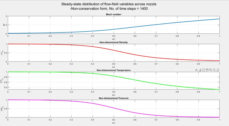
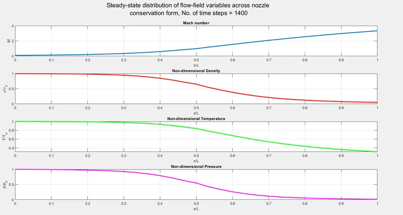
Observation: We can observe that the solution trend obtained in both the forms of the equation are similar.

2. Time-wise variation of the primitive variables

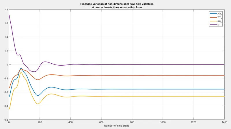
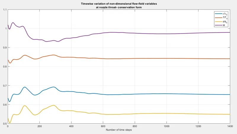
Observation:

• In both the cases the solution converges to the steady state value and it can be further introspected that, in non conservative form the solution converges around 400 time steps and in conservative form the solution converges almost around 550 time steps.
• it can be further seen that the oscillatory behaviour is much lesser in conservative form than non conservative form

Variation of Mass flow rate distribution inside the nozzle at different time steps during the time-marching process

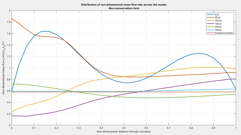
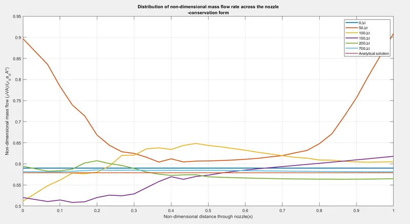
Observation:

• It can be observed that the mass flow rate converges to the steady state value after few time steps. Intially at time steps say till 200*deltat. the solution is flopping up and down. But after the time =200*Deltat, the soltion line flatenning up forming an straight line which is almost close to value of 0.5 (steady state analytical value).
• This behaviour is found in both the cases.

4. Comparison of Normalized mass flow rate distributions of both forms

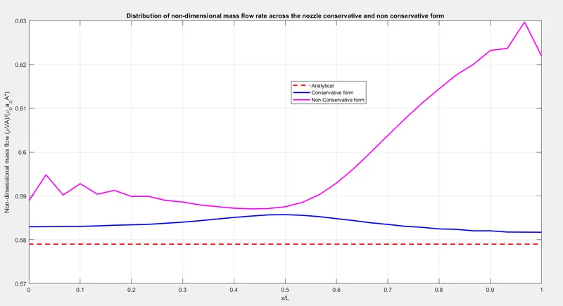
Observation:

On comparing the solution of booth conservative and non conservative form, from the mass flow rate it can be concluded that, its variation

• in conservation form is much closer to the analytical solution when compared to the non conservation form, which have large variations at the inlet and outlet.
• The variation looks quite large but when the results are looked upon from larger time scale the variations look like a straight line. hence one need to be quite careful while interpreting the results.
• The conservation form does better in conserving the mass comapred to the non conservation form as one of the variable of the solution vector was the mass flow rate. where as the non conservation was unable to conserve the mass as mass flow was evalauted after the solution procedure using the primitve variables.

Few other discussions:

Variations of the averaged derivatives with the time step: This is an indicative of the convergence of the method being used:

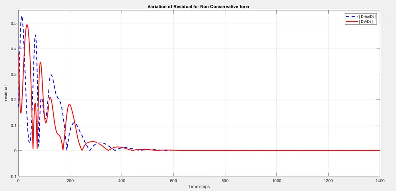
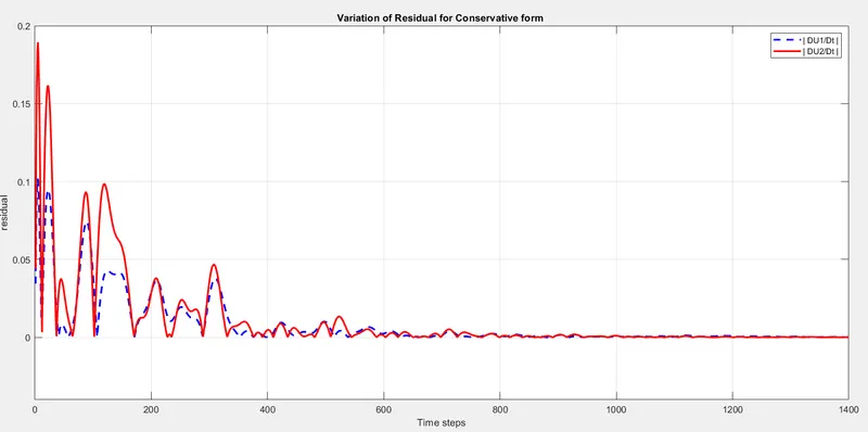
It can be observed that the residual i.e. the RHS of the governing equation comes to zero after the 6oo time steps indicating the convergence of the solution. Many time if we are dealing with multiple methods inorder to appreciate the efficacy of the method the residual plot can be an outstanding parameter

Perform a grid independence test on the solution and expain all your findings.

The grid independence study was performed with the following number of node:

Code was little bit tweaked to obtain the following plots for the grid independence study:

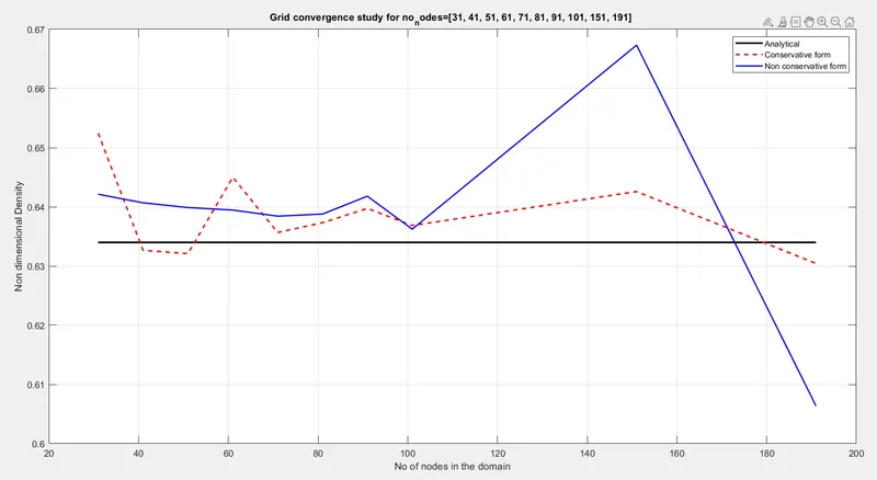
It can be observed that for the variable density, the variation in conservative fom is quite near to the reality, where as with increase in the number of nodes the variation becomes more.

The similar trend was observed with the Mach number and Pressure ratio. The subsequent plots indicate that:

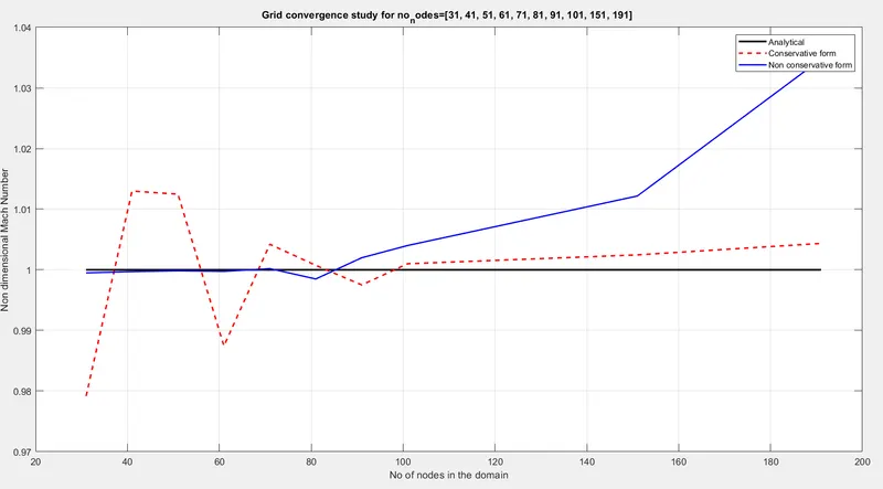
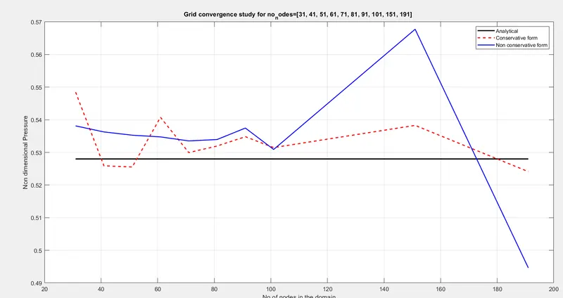
The error can be reduced further by exploring the variation of courant number.

FOr an courant number of 0.8"

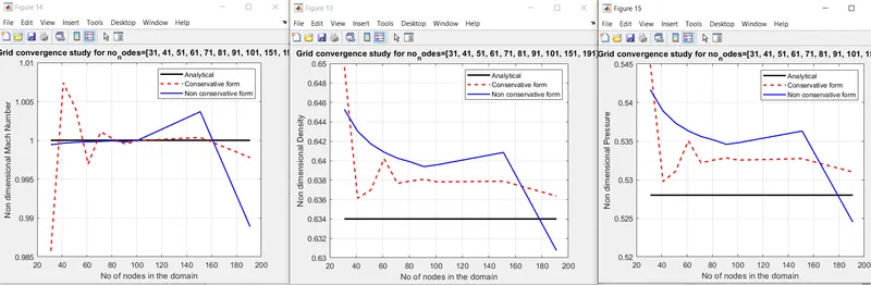
It can be seen that for an higher courant number the conservative form tries to reduce the error with the increase in number of nodes.