Week 11 - Simulation of Flow through a pipe in OpenFoam

In this challenge, you will simulate an axi-symmetric flow by applying the wedge boundary condition. The flow is laminar and flows through a constant cross-section pipe at an inlet Reynold's number of 2100. You can do a transient or steady state simulation and you will validate your results with the Hagen- Poiseuille's equations for the fully developed flow.

You will also write code in Matlab to automate the generation of blockMeshDict file. The code should take inputs like pipe length, diameter, wedge angle, etc and output a fully functional blockMeshDict file.

Expected Results

1. Validate Hydro-dynamic length with the numerical result
2. Validate the fully developed flow velocity profile with its analytical profile
3. Validate maximum velocity and pressured drop for fully developed flow
4. Post-process Shear stress and validate wall shear stress for fully developed flow

Before we go ahead with the simulation its always necessary to revisit the fundamental variables which are involved in the simulation. The once specific variable of interest is the Entrance length.

Entrance Length:

It is defined as that length from the inlet where the boundary layer from the wall is fully developed. After the entrance length the zone is called as fully developed zone. The following thing is shown in the figure below :

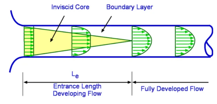
When the boundary layer extends to fill the entire pipe, the flow grows into a fully developed flow where the flow characteristics no longer change with increased distance along the pipe.

Hydrodynamic entrance length:

The hydrodynamic entrance region refers to the area of a pipe where fluid entering a pipe develops a velocity profile due to viscous force spreading from a pipe's interior wall. This region has a non-uniform flow.

When the fluid enters a pipe, fluid particles in the adjacent to the pipe's surface come to a complete stop because of the no-slip condition. The layer adjacent to the first layer moves the flow and hence there is a gradient of velocity in the direction opposite to the flow. In order to estiamte the entrance length we have the corrections corresponding to the inlet reynolds number and diameter of the pipe or hydraulic diamtere of the channel.

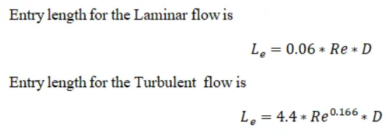ref: Data book by kodhandaraman Heat and mass transfer

Hagen Poiseuille equations

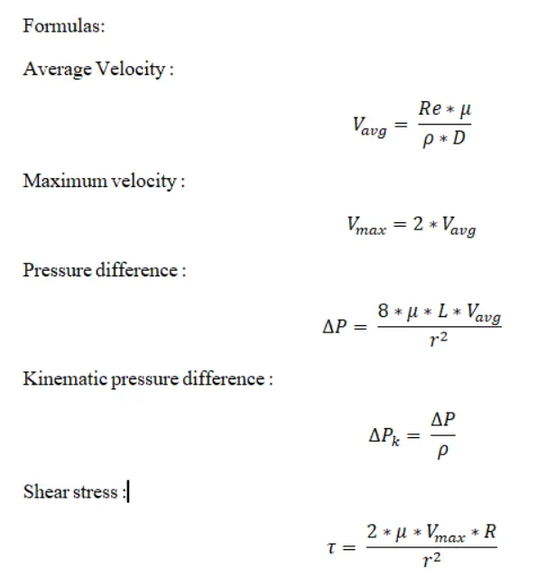
Hagen Poiseuille equations, are the solutions of the flow equations in fully developed region and they cant be applied to the entrance length zone. The following are the equations and can be referred from any std. fluid mechanics book

Given conditions:

Reynolds number(Re) =2100

For the internal flows the reynolds number of 2100 is < 2500 and hence its laminar by nature and icofoam or simple foam can be used as the solver.

Assumed properties:

• Diameter ,D = 0.004
• Radius, r = 0.002
• Radial Distance, R = 0 to r
• Dynamic viscosity, mu = 0.00089 N/m^2
• Density, rho = 997 kg/m^3

Task 1: create an matlab script whcih can create an blockmeshdict file automatically for various values of the wedge angle

The matlab code is attached below:

 clear all
close all
clc
% The Reynolds number
Re = 2100
% The Diameter of pipe
D = 0.004
% The Entry length of pipe
L =0.06*Re*D
% The total length of pipe
L_p = L+0.7
% Radius of pipe
r = D/2
% Angle of wedge (less than 5)
theta = 4
% Dynamic viscosity
mu = 0.89e-3
% Density 
rho = 997
% Hagen poiseuille flow equations
v_avg = (Re*mu)/(rho*D)
v_max = 2*(v_avg)
del_p = (8*mu*L_p*v_avg)/(r^2)
kinematic_p = del_p/rho
% calculating shear stress
R = linspace(0,(D/2),1000)
for i = 1:length(R)
 tau(i) = 2*mu*v_max*(abs(R(i)))/r^2
end
plot(R,tau)
xlabel('Radius')
ylabel('Shear stress')
grid on
legend ('Shear stress')
header1='/*----------------------------------*- C++ -*------------------------------------*\'
header2=' ========= | ' 
header3=' \\ / F ield | OpenFOAM: The Open Source CFD Toolbox '
header4=' \\ / O peration | Website: https://openfoam.org '
header5=' \\ / A nd | Version: 7 '
header6=' \\/ M anipulation | '
header7='\*----------------------------------------------------------------------------------*/'
f1 = fopen('blockMeshDict','w')
fprintf(f1, '%s\n', header1)
fprintf(f1, '%s\n', header2)
fprintf(f1, '%s\n', header3)
fprintf(f1, '%s\n', header4)
fprintf(f1, '%s\n', header5)
fprintf(f1, '%s\n', header6)
fprintf(f1, '%s\n', header7)
fprintf(f1, 'FoamFile\n{\n')
fprintf(f1, '%12s \t 2.0;\n','version')
fprintf(f1, '%12s \t ascii;\n','format')
fprintf(f1, '%12s \t dictionary;\n','class')
fprintf(f1, '%12s \t blockMeshDict;\n','object')
fprintf(f1, '}\n')
header8='// * * * * * * * * * * * * * * * * * * * * * * * * * * * * * * * * * * * * * //'
fprintf(f1, '%s\n\n',header8)
fprintf(f1, 'convertToMeters 1;\n\n')
fprintf(f1, 'vertices\n')
fprintf(f1, '(\n')
fprintf(f1, '\t (%d %d %d)\n',0,0,0)
fprintf(f1, '\t (%d %d %d)\n',0,r*cosd(theta/2),r*sind(theta/2))
fprintf(f1, '\t (%d %d %d)\n',0,r*cosd(theta/2),-r*sind(theta/2))
fprintf(f1, '\t (%d %d %d)\n',L_p,0,0)
fprintf(f1, '\t (%d %d %d)\n',L_p,r*cosd(theta/2),r*sind(theta/2))
fprintf(f1, '\t (%d %d %d)\n',L_p,r*cosd(theta/2),-r*sind(theta/2))
fprintf(f1, ');\n\n')
fprintf(f1, 'blocks\n')
fprintf(f1, '(\n')
fprintf(f1, '\t hex (0 3 5 2 0 3 4 1) (%d %d %d)',300,30,1)
fprintf(f1, ' SimpleGrading (1 0.1 1)\n\n')
fprintf(f1, ');\n\n')
fprintf(f1, 'edges\n')
fprintf(f1, '(\n')
fprintf(f1, '\t arc %d %d (%d %d %d)\n',1,2,0,r,0)
fprintf(f1, '\t arc %d %d (%d %d %d)\n',4,5,L_p,r,0)
fprintf(f1, ');\n\n')
fprintf(f1, 'boundary\n')
fprintf(f1, '(\n')
fprintf(f1, '\t inlet \n')
fprintf(f1, '\t {\n')
fprintf(f1, '\t\t type patch;\n')
fprintf(f1, '\t\t faces\n')
fprintf(f1, '\t\t (\n')
fprintf(f1, '\t\t\t (0 1 2 0)\n')
fprintf(f1, '\t\t );\n')
fprintf(f1, '\t }\n')
fprintf(f1, '\t outlet\n')
fprintf(f1, '\t {\n')

fprintf(f1, '\t\t type patch;\n')
fprintf(f1, '\t\t faces\n')
fprintf(f1, '\t\t (\n')
fprintf(f1, '\t\t\t (3 5 4 3)\n')
fprintf(f1, '\t\t );\n')
fprintf(f1, '\t }\n')
fprintf(f1, '\t top\n')
fprintf(f1, '\t {\n')
fprintf(f1, '\t\t type wall;\n')
fprintf(f1, '\t\t faces\n')
fprintf(f1, '\t\t (\n')
fprintf(f1, '\t\t\t (1 4 5 2)\n')
fprintf(f1, '\t\t );\n')
fprintf(f1, '\t }\n')
fprintf(f1, '\t front\n')
fprintf(f1, '\t {\n')
fprintf(f1, '\t\t type wedge;\n')
fprintf(f1, '\t\t faces\n')
fprintf(f1, '\t\t (\n')
fprintf(f1, '\t\t\t (0 3 4 1)\n')
fprintf(f1, '\t\t );\n')
fprintf(f1, '\t }\n')
fprintf(f1, '\t back\n')
fprintf(f1, '\t {\n')
fprintf(f1, '\t\t type wedge;\n')
fprintf(f1, '\t\t faces\n')
fprintf(f1, '\t\t (\n')
fprintf(f1, '\t\t\t (0 2 5 3)\n')
fprintf(f1, '\t\t );\n')
fprintf(f1, '\t }\n')
fprintf(f1, '\t axis\n')
fprintf(f1, '\t {\n')
fprintf(f1, '\t\t type empty;\n')
fprintf(f1, '\t\t faces\n')
fprintf(f1, '\t\t (\n')
fprintf(f1, '\t\t\t (0 3 3 0)\n')
fprintf(f1, '\t\t );\n')
fprintf(f1, '\t }\n')
fprintf(f1, '); \n\n')
fprintf(f1, 'mergePatchPairs\n')
fprintf(f1, '(\n')
fprintf(f1, ');\n')
header9='// * * * * * * * * * * * * * * * * * * * * * * * * * * * * * * * * * * * * * //'
fprintf(f1, '%s\n',header9)
fclose(f1)

Most of the code is quite self explanatory and the vast majority of the lines used to do file operations i.e. write the a block of line to the file using fprintf command. The file name is pointed to the memory using file pointer f1

The geometry:

In order to fully take the advantage of the symmetry involved in the geometry we use the type called as wedge in the geometry. The geometry developed and the node nomenclature used is as follows:

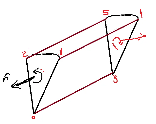
The surface created are:

• 0120 inlet type patch
• 3543 outlet type patch
• 03410 wedge symmetry
• 02530 wedge symmtry
• 1452 wall type wall
• 0330 type symmetry

Note that all the boudaries are created by making sure that normal to the surfaces are pointing in the outward direction.

The blockMesh Dict file created by the matlab code is :

/*----------------------------------*- C++ -*------------------------------------*\
 ========= | 
 \\ / F ield | OpenFOAM: The Open Source CFD Toolbox 
 \\ / O peration | Website: https://openfoam.org 
 \\ / A nd | Version: 7 
 \\/ M anipulation | 
\*----------------------------------------------------------------------------------*/
FoamFile
{
     version 	 2.0;
      format 	 ascii;
       class 	 dictionary;
      object 	 blockMeshDict;
}
// * * * * * * * * * * * * * * * * * * * * * * * * * * * * * * * * * * * * * //

convertToMeters 1;

vertices
(
	 (0 0 0)
	 (0 1.998782e-03 6.979899e-05)
	 (0 1.998782e-03 -6.979899e-05)
	 (1.204000e+00 0 0)
	 (1.204000e+00 1.998782e-03 6.979899e-05)
	 (1.204000e+00 1.998782e-03 -6.979899e-05)
);

blocks
(
	 hex (0 3 5 2 0 3 4 1) (300 30 1) SimpleGrading (1 0.1 1)

);

edges
(
	 arc 1 2 (0 2.000000e-03 0)
	 arc 4 5 (1.204000e+00 2.000000e-03 0)
);

boundary
(
	 inlet 
	 {
		 type patch;
		 faces
		 (
			 (0 1 2 0)
		 );
	 }
	 outlet
	 {
		 type patch;
		 faces
		 (
			 (3 5 4 3)
		 );
	 }
	 top
	 {
		 type wall;
		 faces
		 (
			 (1 4 5 2)
		 );
	 }
	 front
	 {
		 type wedge;
		 faces
		 (
			 (0 3 4 1)
		 );
	 }
	 back
	 {
		 type wedge;
		 faces
		 (
			 (0 2 5 3)
		 );
	 }
	 axis
	 {
		 type empty;
		 faces
		 (
			 (0 3 3 0)
		 );
	 }
); 

mergePatchPairs
(
);
// * * * * * * * * * * * * * * * * * * * * * * * * * * * * * * * * * * * * * //

Boundary condition file:

The P and U files are corrected by providing the boundary names and the types. The pressure and avg velocity calculated from the poiselli flow are used as the initial conditions in these file. The following are sthe files:

/*--------------------------------*- C++ -*----------------------------------*\
  =========                 |
  \\      /  F ield         | OpenFOAM: The Open Source CFD Toolbox
   \\    /   O peration     | Website:  https://openfoam.org
    \\  /    A nd           | Version:  9
     \\/     M anipulation  |
\*---------------------------------------------------------------------------*/
FoamFile
{
    format      ascii;
    class       volVectorField;
    location    "0";
    object      U;
}
// * * * * * * * * * * * * * * * * * * * * * * * * * * * * * * * * * * * * * //

dimensions      [0 1 -1 0 0 0 0];

internalField   uniform (1 0 0);

boundaryField
{
 inlet
 {
 type fixedValue;
 value uniform (0.4686 0 0);
 }
 outlet
 {
 type zeroGradient;
 }
 axis
 {
 type empty;
 }
 top
 {
 type fixedValue;
 value uniform (0 0 0);
 }
 front
 {
 type wedge;
 }
 back
 {
 type wedge;
 }
}
// ************************************************************************* //

/*--------------------------------*- C++ -*----------------------------------*\
  =========                 |
  \\      /  F ield         | OpenFOAM: The Open Source CFD Toolbox
   \\    /   O peration     | Website:  https://openfoam.org
    \\  /    A nd           | Version:  9
     \\/     M anipulation  |
\*---------------------------------------------------------------------------*/
FoamFile
{
    format      ascii;
    class       volScalarField;
    location    "0";
    object      p;
}
// * * * * * * * * * * * * * * * * * * * * * * * * * * * * * * * * * * * * * //

dimensions      [0 2 -2 0 0 0 0];

internalField   uniform 0;

boundaryField
{
 inlet
 {
 type zeroGradient;
 }
 outlet
 {
 type fixedValue;
 value uniform 1.0073;
 }
 axis
 {
 type empty;
 }
 top
 {
 type zeroGradient;
 }
 front
 {
 type wedge;
 }
 back
 {
 type wedge;
 }
}
// ************************************************************************* //

ControlDict File:

/*--------------------------------*- C++ -*----------------------------------*\
  =========                 |
  \\      /  F ield         | OpenFOAM: The Open Source CFD Toolbox
   \\    /   O peration     | Website:  https://openfoam.org
    \\  /    A nd           | Version:  9
     \\/     M anipulation  |
\*---------------------------------------------------------------------------*/
FoamFile
{
    format      ascii;
    class       dictionary;
    location    "system";
    object      controlDict;
}
// * * * * * * * * * * * * * * * * * * * * * * * * * * * * * * * * * * * * * //

application     icoFoam;

startFrom       startTime;

startTime       0;

stopAt          endTime;

endTime         1;

deltaT          0.001;

writeControl    timeStep;

writeInterval   20;

purgeWrite      0;

writeFormat     ascii;

writePrecision  6;

writeCompression off;

timeFormat      general;

timePrecision   6;

runTimeModifiable true;


// ************************************************************************* //

Open foam procedure (with paralle computing)

The following commands are used in the console to solve the problem. Make sure that

command: blockMesh

• firstly the blockMesh command will be run to make sure that the mesh is reconstructed and the polymesh file is created which can be used for solving.

command: decomposePar

• it decomposes the geometery based on the number of cores i.e. 4 in my case. This is a vital piece of command and inorder to do it you need to make sure that you have the decomposebarDict file in the system folder.

command: mpirun -np 4 icoFoam -parallel > log&

• This statement says the system to run the icofiam solver in the parallel mode. np here indicates the number of cores used for the parallel computing.
• icofoam > loag & is used if you want to store the data to the log file and the log& and symbol allows the open foam to run in the background giving us the opportunity to type extra lines of code in the console

command: foamLog log

• This statement says the system to create an individual log files from the single log files for the variables being solved
• These are very useful as they can be exported to excel. matlab for further processing

command: gnuplot residual.txt

• This statement tells matlab to plot the residual with the help of the code written in the file called residual.
• in order to be able to use this you need a small part of code which has to be stored in the same folder or dierctory
• The code is:

set logscale y
set title "Residuals"
set ylabel 'Residual'
set xlabel 'Iteration'
plot "< cat log | grep 'Solving for Ux' | cut -d' ' -f9 | tr -d ','" title 'Ux' with lines,\
"< cat log | grep 'Solving for Uy' | cut -d' ' -f9 | tr -d ','" title 'Uy' with lines,\
"< cat log | grep 'Solving for Uz' | cut -d' ' -f9 | tr -d ','" title 'Uz' with lines,\
"< cat log | grep 'Solving for p' | cut -d' ' -f9 | tr -d ','" title 'p' with lines
pause 1
reread

There are plenty of videos on this on youtube and code is also available

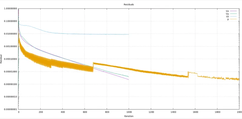
This is how the residual plots looks like and the.

command: reconstructPar

• This statement tells the openfoam to recombine the solutions from all the 4 cores used and in this stage you will find that the induvidual folders at various time stepsa are created. This is a bit time taking process but never less parallel run time will be very less compared to the serial

command: ParaFoam

• Used to open the paraview and view the results.

Geometry visualization:

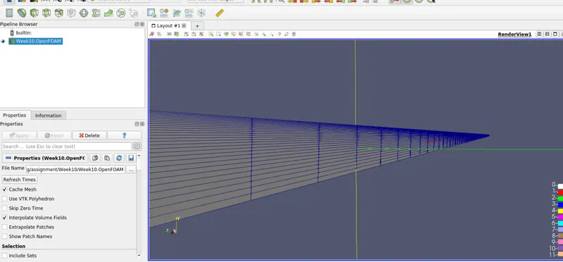
The velocity contour

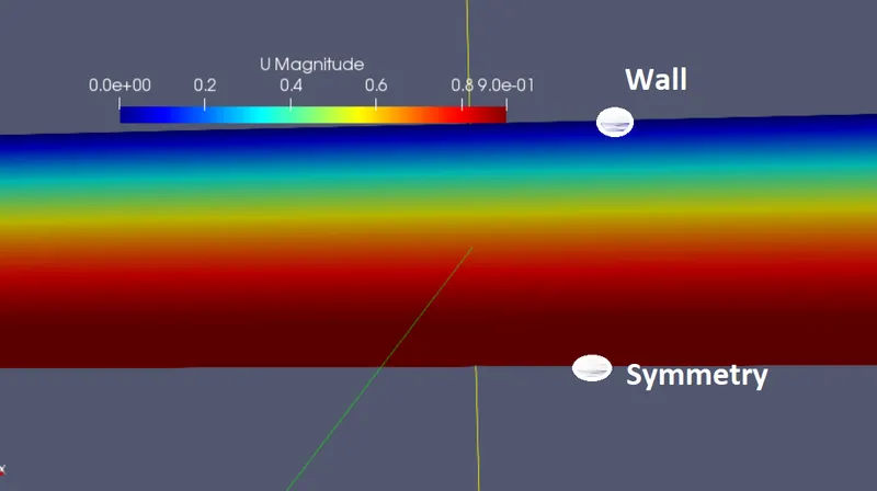
It can be seen that:

• Velocity is zero at the wall due to no slip condition and
• Velocity is max at the symmetry as it is the centre of the pipe

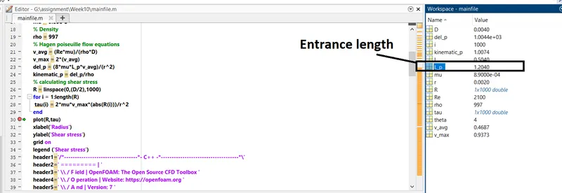
Validate Hydro-dynamic length with the numerical result

as per the analytical formulae the Entrance length is : 1.204

Variation of the pressure along the length:

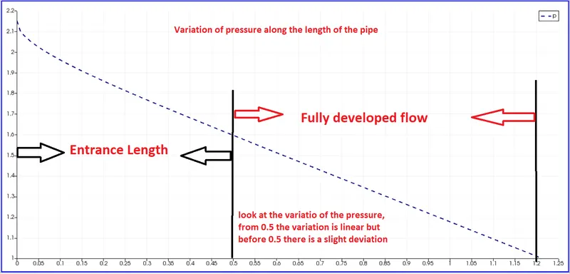
In order to calculate the Entrance length we need the velocity, and hence let us plot the velocity profiles at various locations along the pipe.

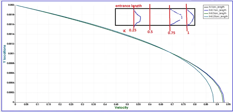
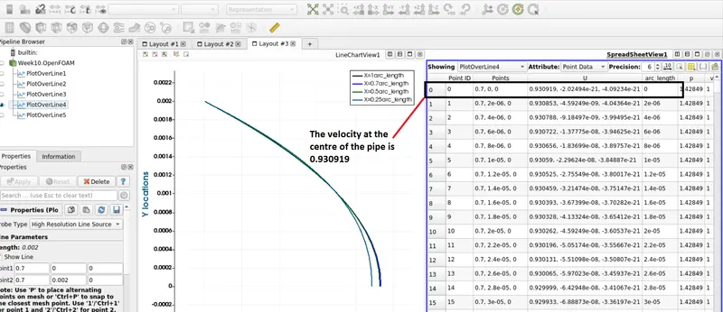
Comparison of the velocity :

Parameter	Value
Velocity_centre_analytical	0.9347
Velocity_centre_CFD	0.930919

`L_e= 0.06*Re*D`

Graphical Evaluation

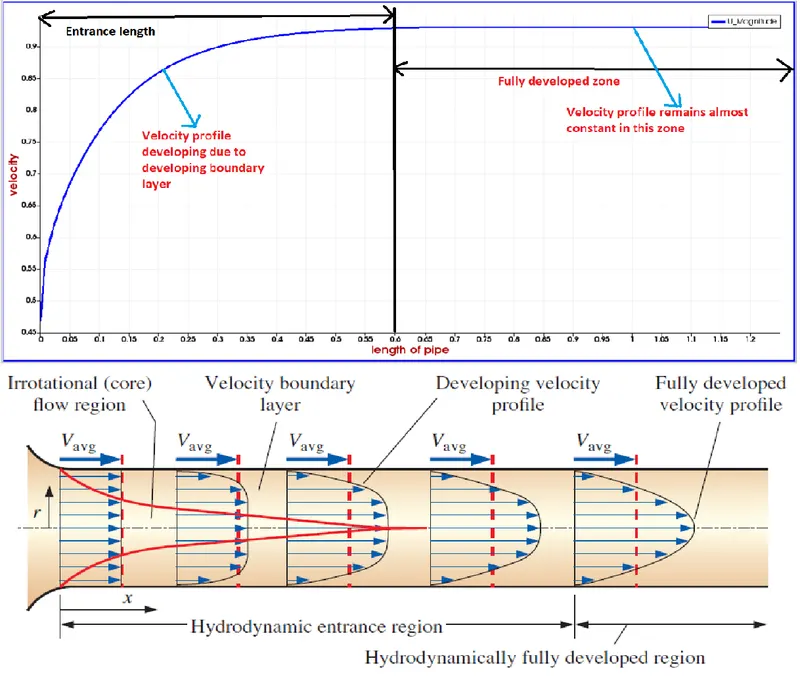
In the fully developed zone the velocity is constant and it is found that this typically happens after the length of X=0.64. Refrer: https://sites.pitt.edu/~sts106/MEMS1071_CFD_Project.pdf

Parameter	Value
Entrance length_analytical	0.5040
Velocity_centre_CFD	0.54

Note: This error can will come down if the mesh refinement is performed

Validate the fully developed flow velocity profile with its analytical profile

small bits of code was written in matlab and the data was imported from excel sheets to make the plot.

The velocity profile _CFD was exported from the paraview to excel sheet and that sheet was imported in matlab.

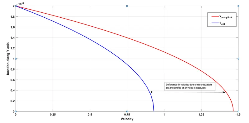
The difference in the velocity is due to coarse mesh and another point to be noted is that analytical solution is same everywhere in the fully developed zone where as when we take the cfd solution the value will change slightly. The CFD solution has captured the physics properly and the error can be further reduced by mesh refinement.

Post-process Shear stress and validate wall shear stress for fully developed flow

Shear can be found from the following piece of code written in matlab:

R = arc_length;
v_max=0.9347;
 %calculating shear stress
 
 for i = 1:length(R)
 tau_ana(i) = 2*mu*v_max*(abs(R(i)))/0.002^2;
end

  % calculating shear stress
dR = R(2)-R(1);
for i = 1:length(R)-1
 du = v_cfd(i+1)-v_cfd(i);
 dU = abs(du);
 tau_cfd(i) = mu*(dU/dR);
end

figure(2)
plot(R(2:end),tau_cfd, 'r', 'LineWidth' ,2)
hold on 
plot(R, tau_ana, '--b', 'LineWidth', 2)

xlabel('Radius')
ylabel('Shear stress')
grid on
legend('\tau_{cfd}', '\tau_{analytical}')

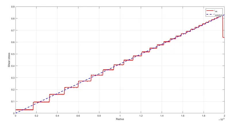
The shear follows the tred as analytical and the maximum shear is near the wall, as the velocity gradient is high near the wall due to no slip condition.

the step profile in cfd is due to the assumption of the step profile made in the finite volume approximation.

Conclusion :

The open foam simulation of the flow through pipe was performed and the essential parameters such as entrance length, maximum velocity. pressure and the shear were compared and the comments are made.