Week 9: Project 1 - Surface preparation and Boundary Flagging (PFI)

Aim: Surface preparation and Boundary Flagging of IC engine geometry and running no hydro simulation.

Objective:

• Performing a no hydro simulation for IC engine.

Introduction:

No hydro simulation is one in which we will not be solving any governing equation but will generate a mesh for the whole body.

This simulation is performed to check whether the body has the right mesh, and the motion profiles added work perfectly such that we can continue with hydrodynamic simulation.

Steps:

• Starting with importing the ICE engine STL file.
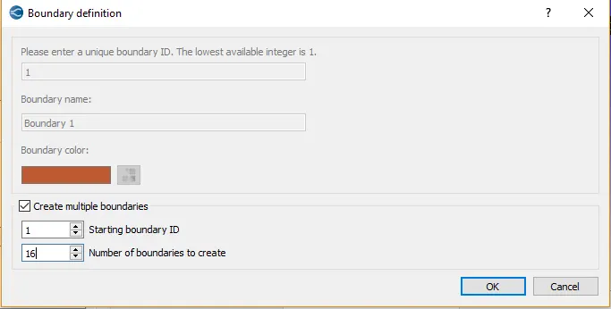
• Defining the number of boundaries to be flagged.

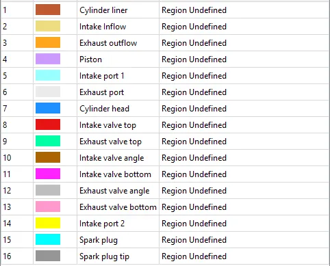
• Assigning the suitable boundary names.

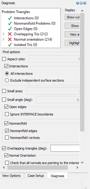
• Surface cleaning in this process we should go to diagnosis dock and click find and we will get a set of errors if the boundary as any.

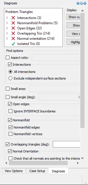
Intersection error:

If two or more lines intersect each other we generally get intersection errors.

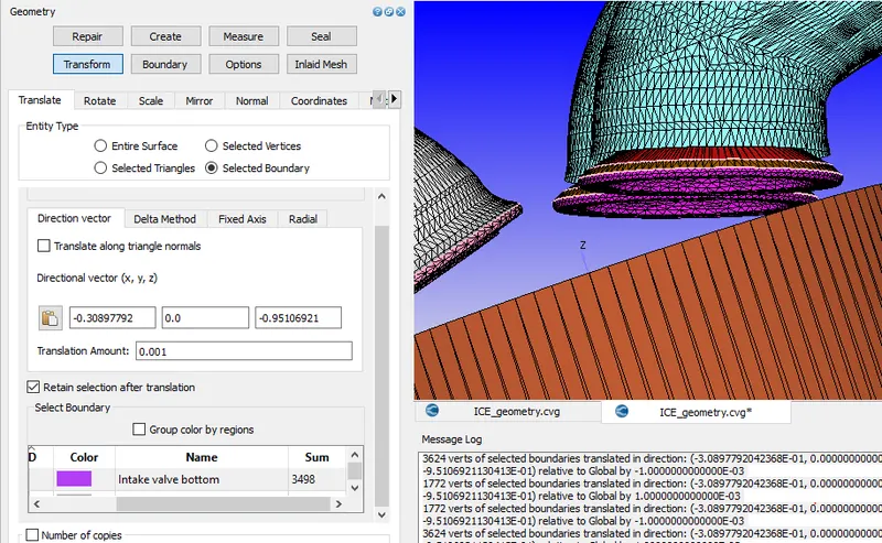
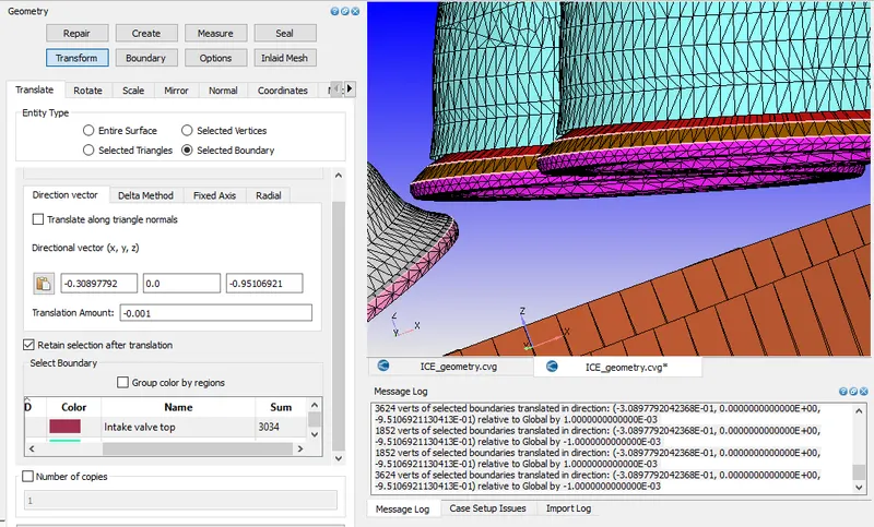
In our geometry, we generally see that the valve body intersects with the cylinder head. To resolve this error, we translate the valve body using translate by boundary command and provide the translation amount and arc normal.

This will resolve intersection errors.

Open Edges:

In this error, we generally see there are voids inside the geometry and to fill them we use the patch command. this will solve most of the errors.

Normal orientation:

The normals of some boundaries are not aligned in the same direction, we can use the transform normal command to select any triangle and change the normal direction.

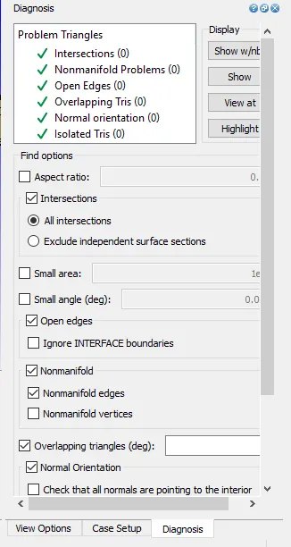
All the errors get resolved now we can move with our case setup.

Case setup:

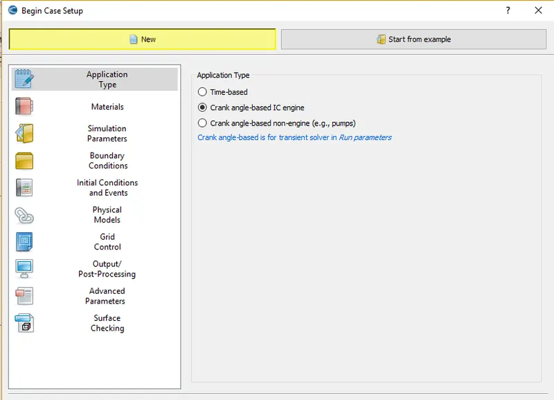
• The application type is crank-angle-based since we are performing IC engine simulation.

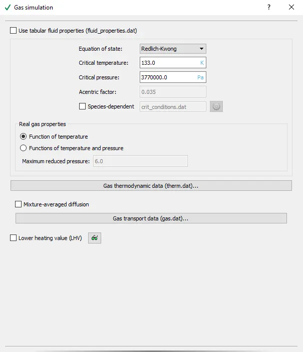
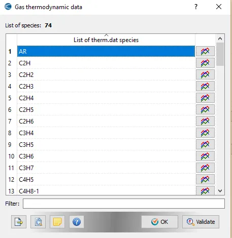
• In the Gas simulation, we should import the therm.dat file for our specified fuel which is Iso-octane (IC8H18).

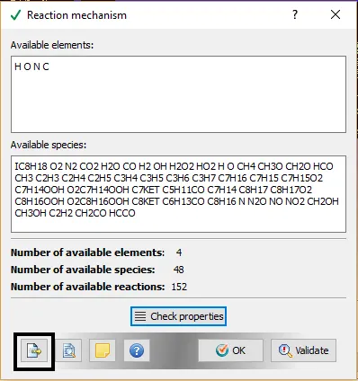
• In the reaction mechanism, we will import the mech.dat file into our case setup.
• To import any file we can click on the bottom left symbol which is been highlighted by the black box in the below image.

Run parameter:

• Transient state simulation which is based on crank angle and mode is no hydro.

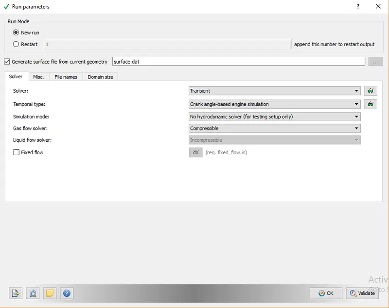
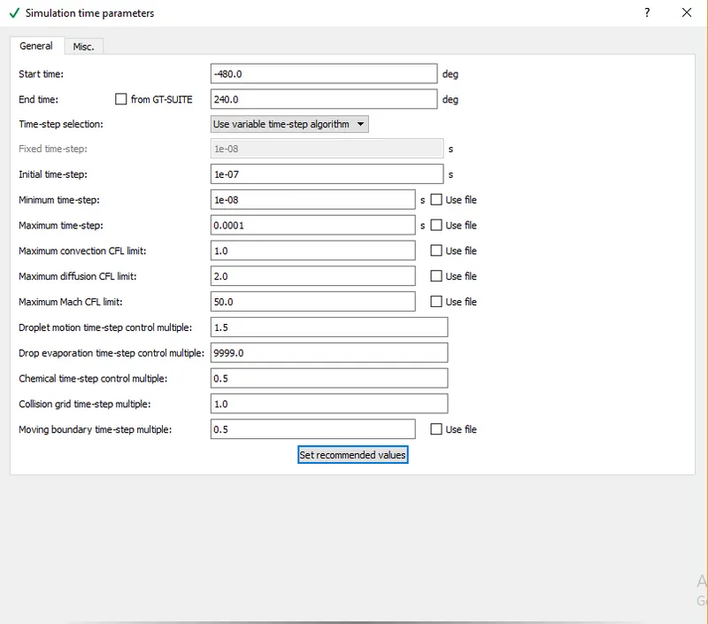
• In simulation time parameters we add start angle and end angle in degree, since one cycle consists of 720 degrees the difference between start and end time must be 720degrees.

Boundaries:

There are many boundaries in the IC engine simulation we will discuss important ones.

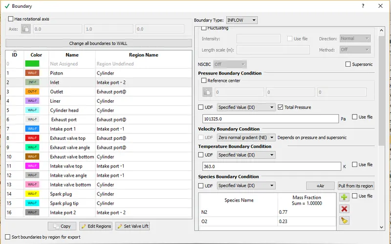
Inlet:

Boundary type: Inflow

Pressure: 1 bar

Temperature: 363K (generally low at intake)

Species: Air

Outlet:

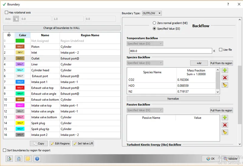
Boundary type: Outflow

Pressure: 1 bar

Temperature: 800K (Higher at exhaust)

Species:

The fuel we are using is iso-octane.

For the selection of species, we will write a stoichiometric equation for the reaction of iso-octane with air.

C₈H₁₈ + ar*(O₂ + 3.76*N₂) = aCO₂ + bH₂O+ ar*3.76*N₂

Molecules	LHS	RHS
C	8	a
H	18	2b
O2	2ar	2a+b

Now from above table we have 3 unknowns with 3 equation hence solution for unknowns are:

a = 8

b = 9

ar = 12.5

Final equation:

C₈H₁₈ + 12.5*(O₂ + 3.76*N₂) = 8CO₂ + 9H₂O+ 47*N₂

In the case of outflow, we are interested in products of the above stoichiometric reactions.

Converge takes the value in terms of the mass fraction so we should calculate the mass fraction of each product species and the sum of the mass fraction should always be ‘1’.

Products:

Molecules	Molecular weight	No of moles	The total mass of each molecule	Mass fractions
CO2	12+32 = 44	8	352	0.19235
H2O	2+16 = 18	9	162	0.08852
N2	28	47	1316	0.71912
		Total mass	1830	1

Piston:

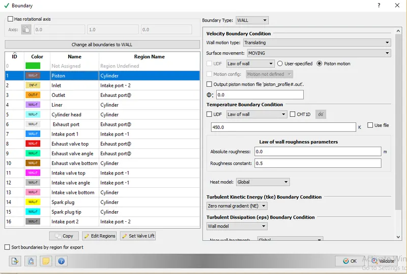
Boundary type: Wall

Motion: Translating

Temperature: 450K

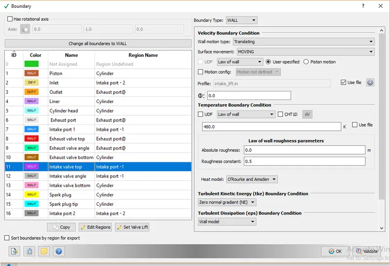
Intake valve:

Boundary type: Wall

Motion: Translating

Profile: We will import an intake_lift.in file.

Temperature: 480K

The intake valve is divided into three parts intake top, intake angle, and intake bottom. For all the boundaries same boundary conditions are applied as shown above.

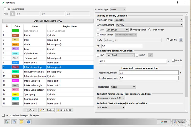
Exhaust valve:

Boundary type: Wall

Motion: Translating

Profile: We will import an Exhaust_lift.in the file.

Temperature: 425K

The intake valve is divided into three parts intake top, intake angle, and intake bottom. For all the boundaries same boundary conditions are applied as shown above.

Regions:

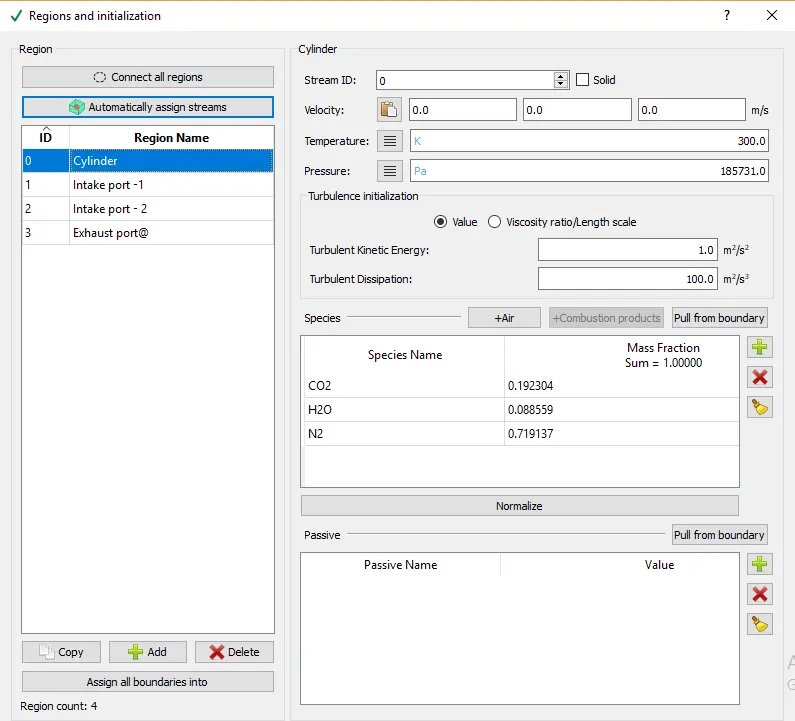
Cylinder region:

Pressure: 1.85 bar

Species: Products derived from the above-mentioned reactions and their mass fraction.

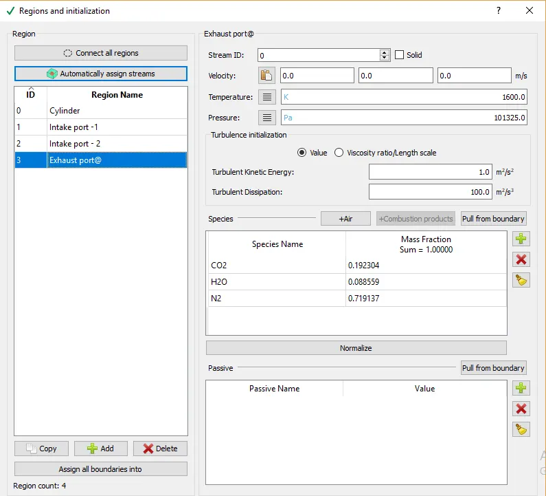
Exhaust port region:

Pressure: 1 bar

Species: Products derived from the above-mentioned reactions and their mass fraction.

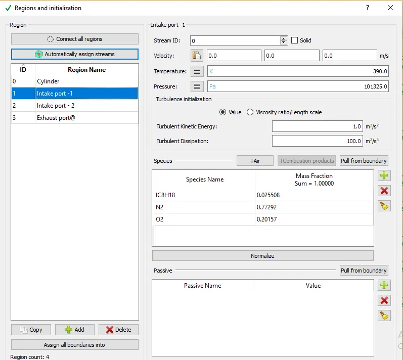
Intake port 1 region:

Pressure: 1 bar

Species:

When fuel is injected into the intake port we will use reactants so it’s important to calculate the mass fraction of reactants too.

Reactants-

Molecules	Molecular weight	No of moles	The total mass of each molecule	Mass fractions
C8H18	114	1	114	0.06229
O2	32	12.5	400	0.21857
N2	28	47	1316	0.71912
		Total mass	1830	1

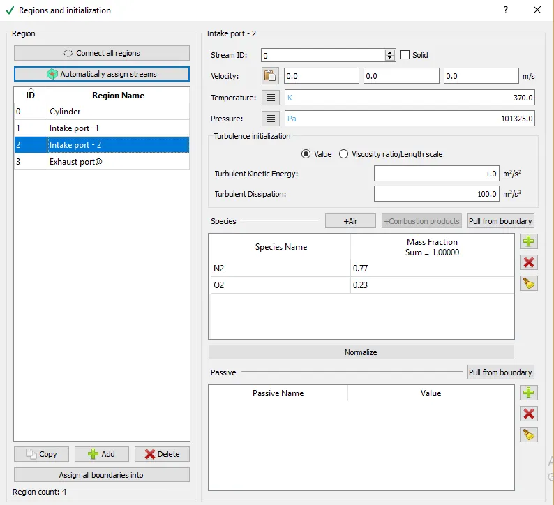
Intake port 2 region:

Pressure: 1 bar

Species: Air

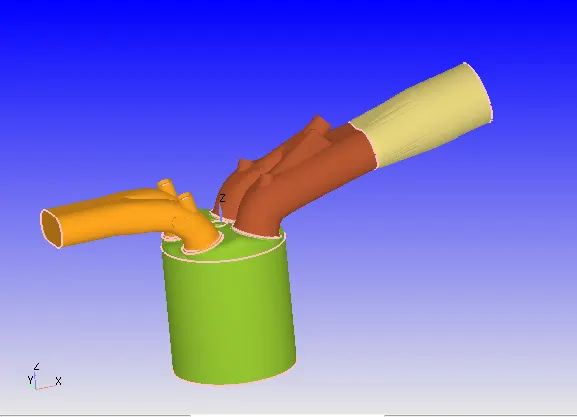
Final IC engine geometry differentiated with regions:

Events:

Cyclic events:

We generally have two cyclic events, events are generally specified for the start of a certain process in between two regions, In this simulation, we have to translatory motion of valves which must be defined in the cyclic event and the lift.in files will be automatically taken care of if they are defined in boundaries.

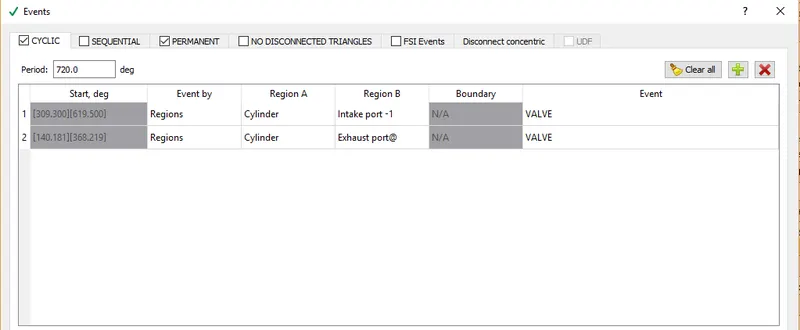
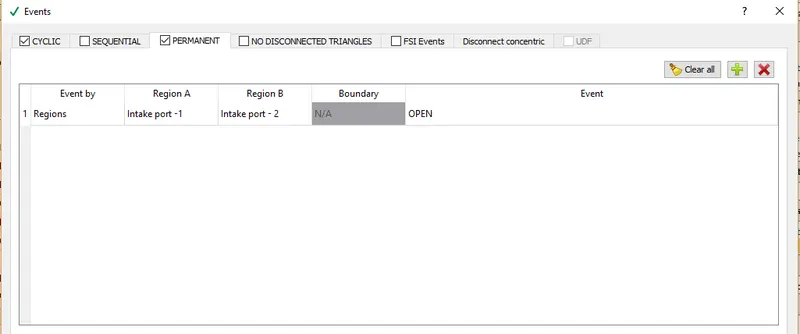
Permanent event:

It is between the intake port-1 and intake port-2 and is always open.

Base grid:

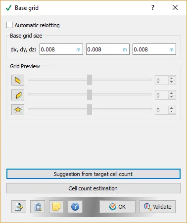
We can apply any size but for no hydro simulation, it is recommended to choose a smaller size since we just want to check whether our mesh and embedding are working well and are changing with the motion of the valve.

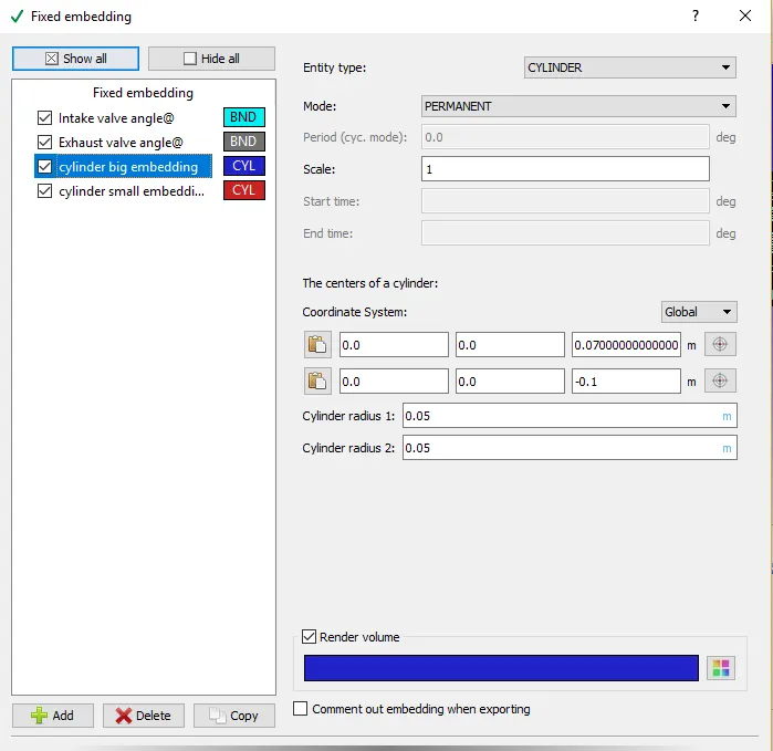
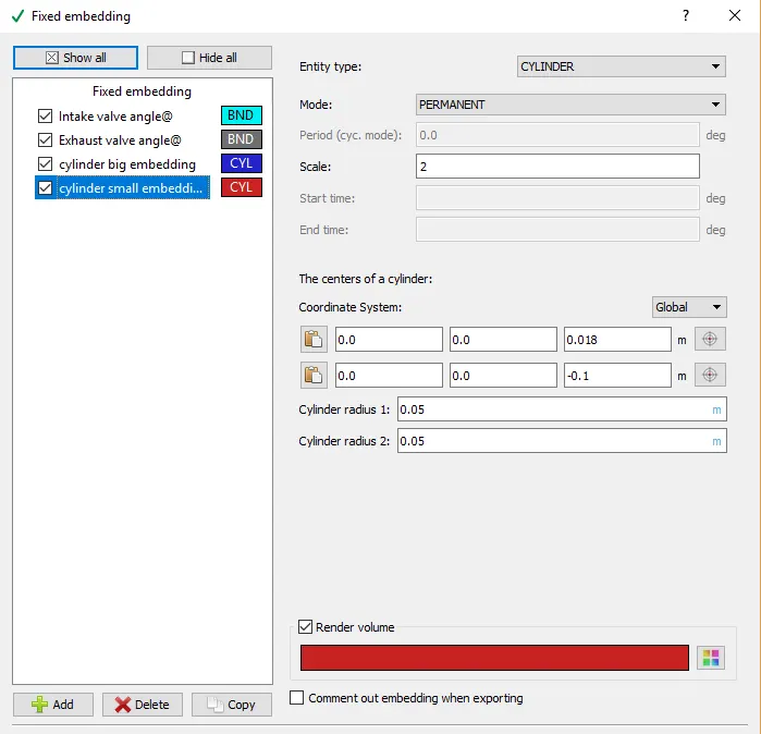
Fixed embedding:

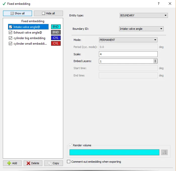
Embedding for intake valve angle:

We apply embedding scale to the boundary of the valves and the assumption is the cell size should be 40% of the base cell size near the walls such that cell paring takes place.

Mode: permanent

Scale: 4

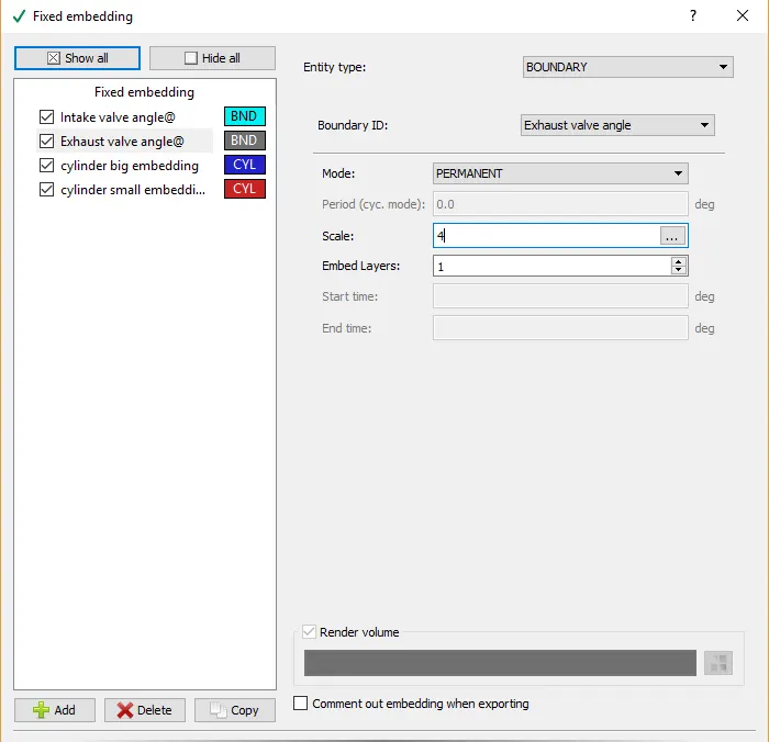
Embedding for exhaust valve angle:

Mode: permanent

Scale: 4

Cylinder big embedding:

Mode: permanent

Scale: 1

Cylinder small embedding:

Mode: permanent

Scale: 2

• For output files, nothing is changed.
• Export the input files and run the simulation using Cygwin.

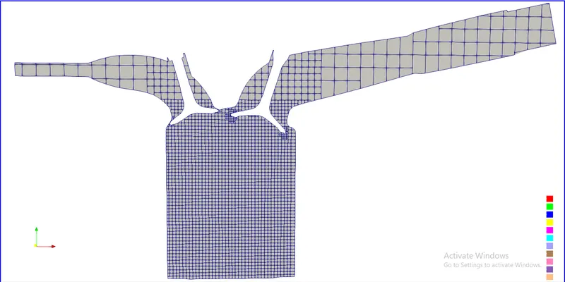
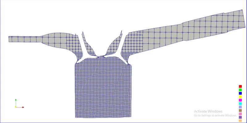
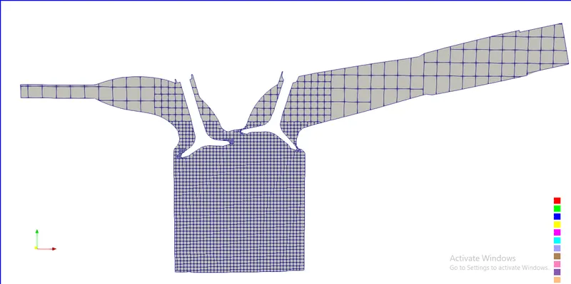
Mesh at different time steps:

Total I have 360-time steps for 1 cycle which consist of 720 degrees rotation.

Time step 0:

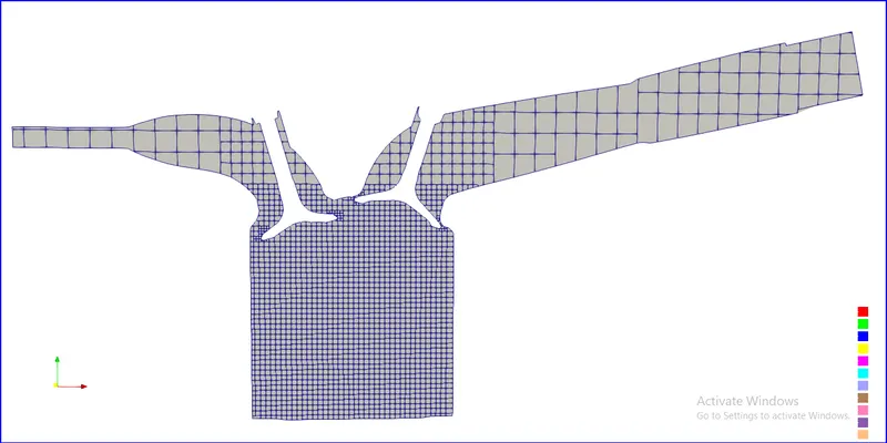
In the above-sliced view, we can find all the embedding scale we defined for different regions.

Time step 50:

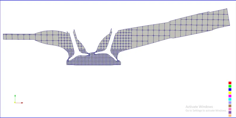
This image represents the piston as moved upward and the exhaust valve has been closed and we can see the refined mesh at the boundaries of the valve.

Time step 150:

Time step 300:

Time step 360:

Video link:

https://drive.google.com/file/d/1QYnOmuYkD_83gR799gyub0svbDmY7sQp/view?usp=sharing